Functional Scoring Metrics¶

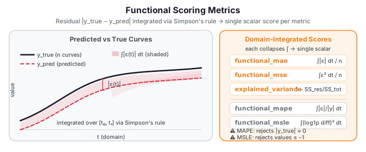
Evaluating functional predictions requires metrics that respect the continuous nature of the data. fdars.scoring provides five domain-integrated prediction-scoring functions: functional_mae, functional_mse, functional_mape, functional_msle, and functional_explained_variance. All share the same uniform signature and return a single scalar.

Functional scoring metrics — concept diagram

Why functional metrics?¶

Scalar regression metrics applied column-wise to a functional dataset (e.g., averaging per-grid-point MSE) treat each evaluation point as equally important regardless of grid spacing. fdars.scoring integrates the error over the domain using Simpson's rule, giving a domain-weighted scalar that properly accounts for non-uniform grids.

For \(n\) pairs of true and predicted curves with shared evaluation grid \(t_1, \ldots, t_m\):

\[ \text{functional\_mae} = \frac{1}{n} \sum_{i=1}^{n} \int_{t_1}^{t_m} \bigl|y_{\text{true},i}(t) - y_{\text{pred},i}(t)\bigr|\, dt \]

\[ \text{functional\_mse} = \frac{1}{n} \sum_{i=1}^{n} \int_{t_1}^{t_m} \bigl(y_{\text{true},i}(t) - y_{\text{pred},i}(t)\bigr)^2\, dt \]

Each integral is approximated via Simpson's rule over the argvals grid. A model that performs badly over a wide domain region is penalised more than one with a narrow spike error — unlike a simple column-wise average.

The five metrics¶

functional_mae¶

Mean absolute integrated error. Robust to outlier curves; same units as the data.

functional_mse¶

Mean squared integrated error. Penalises large errors more heavily; squared units.

functional_explained_variance¶

\[ \text{EV} = \frac{1}{n} \sum_{i=1}^{n} \Biggl(1 - \frac{\int(\varepsilon_i(t) - \bar\varepsilon_i)^2\,dt}{\int(y_{\text{true},i}(t) - \bar y_{\text{true},i})^2\,dt}\Biggr) \]

where \(\varepsilon_i = y_{\text{true},i} - y_{\text{pred},i}\) and bars denote per-curve means. Range: \((-\infty, 1]\). A value of 1 means the model explains all variation; values near or below 0 indicate a poor fit.

functional_mape¶

Mean absolute percentage integrated error:

\[ \text{MAPE} = \frac{1}{n} \sum_{i=1}^{n} \int_{t_1}^{t_m} \frac{|y_{\text{true},i}(t) - y_{\text{pred},i}(t)|}{|y_{\text{true},i}(t)|}\, dt. \]

MAPE raises on near-zero truths

functional_mape raises ValueError when any |y_true(t)| < ε for any curve and any grid point (no epsilon-in-denominator fallback — the library correctly rejects inputs near zero rather than producing numerically undefined results). Do not use MAPE on data that crosses or approaches zero. For zero-crossing data, use functional_mae or functional_mse instead. For non-negative data, functional_msle is a better relative-error metric.

functional_msle¶

Mean squared log-error:

\[ \text{MSLE} = \frac{1}{n} \sum_{i=1}^{n} \int_{t_1}^{t_m} \bigl(\ln(1 + y_{\text{true},i}(t)) - \ln(1 + y_{\text{pred},i}(t))\bigr)^2\, dt. \]

MSLE raises when any value ≤ −1

functional_msle raises ValueError when any value in y_true or y_pred is ≤ −1 (since \(\ln(1 + v)\) is undefined at \(v = -1\)). Ensure all values are strictly greater than −1 before calling this metric.

Uniform signature¶

All five functions share the same call signature:

from fdars.scoring import (
    functional_mae,
    functional_mse,
    functional_mape,
    functional_msle,
    functional_explained_variance,
)

score = functional_mae(y_true, y_pred, argvals)  # same for the other four

Parameter	Type	Description
`y_true`	`ndarray (n, m)`	True functional observations; rows are curves
`y_pred`	`ndarray (n, m)`	Predicted functional observations; must have the same shape
`argvals`	`ndarray (m,)`	Shared evaluation grid; used for Simpson integration weights

Returns: Python float — the curve-averaged integrated score.

Worked example¶

The fence below uses the Tecator NIR absorbance dataset (240 spectra, 100 wavelength channels, all values positive) as a predict-vs-true setup. The cross-sectional mean is used as a baseline predictor — anything informative should beat it. All three domain-safe metrics are demonstrated; MAPE and MSLE are described in prose only because their domain restrictions are documented above.

import numpy as np
from docs_data import load_tecator
import fdars.fdata as ff
from fdars.scoring import (
    functional_mae,
    functional_mse,
    functional_explained_variance,
)

wl, X, meta = load_tecator()
# X: 240 spectra × 100 wavelength channels, values in [2, 5.5] (positive — safe for all metrics)
# Use 12 held-out curves as y_true; predict each with the training-set mean (baseline)
rng = np.random.default_rng(42)
idx = rng.choice(len(X), size=12, replace=False)
y_true = X[idx]

# Baseline: predict the overall mean for every curve (deliberately uninformative)
mean_curve = np.asarray(ff.mean_1d(X))
y_pred = np.tile(mean_curve, (12, 1))

mae = functional_mae(y_true, y_pred, wl)
mse = functional_mse(y_true, y_pred, wl)
ev  = functional_explained_variance(y_true, y_pred, wl)

print(f"Dataset:              Tecator NIR spectra (n=12, m={X.shape[1]})")
print(f"Baseline predictor:   cross-sectional mean (worst-case uninformative)")
print(f"functional_mae:       {mae:.4f}  (integrated absolute error)")
print(f"functional_mse:       {mse:.4f}  (integrated squared error)")
print(f"explained_variance:   {ev:.4f}  (1 = perfect; 0 = mean-level)")
print(f"FDARS_FENCE_OK")

Dataset: Tecator NIR spectra (n=12, m=100) Baseline predictor: cross-sectional mean (worst-case uninformative) functional_mae: 64.8805 (integrated absolute error) functional_mse: 33.6711 (integrated squared error) explained_variance: 0.9644 (1 = perfect; 0 = mean-level) FDARS_FENCE_OK

Metric comparison¶

The five metrics have different units, domain restrictions, and sensitivity profiles. Use this table to select the right metric before fitting a model.

Metric	Units	Domain restriction	Outlier robustness	Typical use
`functional_mae`	Same as data	None	High — linear in error	General purpose; error reporting in original units; robust baseline
`functional_mse`	Data²	None	Low — squares large errors	Model selection when large deviations matter most; gradient-based optimisation
`functional_explained_variance`	Dimensionless (−∞, 1]	None	Moderate	Variance-explained reporting; comparing models on the same dataset; 1 = perfect
`functional_mape`	Percentage	`\\|y_true(t)\\| > 0` everywhere	Low — denominator near 0 inflates	Relative error on strictly positive functional data (spectra, counts above zero)
`functional_msle`	Dimensionless	All values > −1	Moderate	Non-negative counts with exponential growth (log scale); penalises underprediction more than overprediction

Choosing the right metric by use case

General purpose / no domain restriction: functional_mae or functional_mse. Start here when unsure.
Reporting error in the original measurement unit: functional_mae — same units as the data, directly interpretable.
Model selection emphasising large deviations: functional_mse — squared error disproportionately penalises outlier curves.
Variance-explained reporting: functional_explained_variance — interpretable scale (0 to 1 for non-negative fits); negative values indicate the predictor is worse than predicting the mean.
Relative error on strictly positive functional data (NIR spectra, non-negative concentrations, demand curves above zero): functional_mape — but only when you can guarantee |y_true(t)| > 0 everywhere across every curve and every grid point. It raises ValueError otherwise.
Non-negative counts or exponential-scale data: functional_msle — the log transform compresses large values and makes the metric less sensitive to extreme over-predictions. Requires all values > −1.
Zero-crossing data, oscillating residuals: avoid functional_mape and functional_msle; use functional_mae or functional_mse.

functional_mape: the |y_true| ≠ 0 requirement is per cell

functional_mape raises ValueError when any single cell y_true[i, j] satisfies |y_true[i, j]| < ε — not just the curve average. A functional curve that crosses zero at even one grid point is enough to cause an error. The danger admonition in the metric definition above is not a soft warning; it is an exact constraint enforced at runtime by the library.

References¶

Ramsay, J.O., Silverman, B.W. (2005). Functional Data Analysis, 2nd ed. Springer.
Ferraty, F., Vieu, P. (2006). Nonparametric Functional Data Analysis. Springer.