Interval-wise Testing Procedure (ITP)¶

The Interval-wise Testing Procedure (ITP) tests where along the domain two functional populations differ — or where a single functional population deviates from a reference curve — with rigorous interval-wise family-wise error rate (FWER) control. Rather than producing a single p-value for the whole domain, ITP returns a vector of p-values, one per basis function, identifying which basis coefficients drive the difference. The fdars.inference module exposes three ITP entry points:

Function	Question answered
`itp_one_pop`	Does the functional mean equal a reference curve \(\mu_0\)?
`itp_two_pop`	Do two functional populations share the same mean curve?
`itp_flm`	Is the functional predictor significant in a scalar-on-function regression?

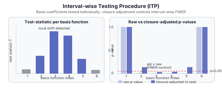
Diagram¶

Interval-wise Testing Procedure — per-basis p-value vector with closure adjustment

Theory¶

Basis expansion and projection¶

Each observed curve \(X_i(t)\) is projected onto a set of \(K\) basis functions \(\{\phi_1, \dots, \phi_K\}\) (B-spline or Fourier), giving scalar coefficients \(c_{ik} = \langle X_i, \phi_k \rangle\). Testing proceeds separately on each coefficient:

\[ H_0^{(k)} : \mathbb{E}[c_{ik}] = c_k^{(0)}, \quad k = 1, \dots, K. \]

For each coefficient \(k\), a permutation null distribution is built by randomly shuffling group labels (or adding/removing the reference function) and recomputing the test statistic. The raw p-value for basis \(k\) is

\[ p_k^{\mathrm{raw}} = \frac{\#\{T_k^* \ge T_k^{\mathrm{obs}}\} + 1}{n_{\mathrm{perm}} + 1}. \]

Closure adjustment and FWER control¶

Because \(K\) hypotheses are tested simultaneously, ITP applies the closure principle to control the interval-wise FWER. The closure adjustment takes cumulative min-p values across nested subsets of basis indices, then re-applies the marginal distribution, producing adjusted p-values \(p_k^{\mathrm{adj}}\) that satisfy

\[ P\!\Bigl(\exists\, k \in S : p_k^{\mathrm{adj}} \le \alpha \;\Big|\; H_0^{(k)} \text{ true for all } k \in S\Bigr) \le \alpha \]

for every subset \(S \subseteq \{1, \dots, K\}\) simultaneously.

Closure increases individual p-values

The adjusted p-values are at or above the raw p-values: \(p_k^{\mathrm{adj}} \ge p_k^{\mathrm{raw}}\). This is the expected behaviour of a multiple-testing correction — the price paid for simultaneous FWER control is that individual coefficients need a stronger signal to be declared significant after adjustment. A coefficient whose raw p-value is 0.005 may have an adjusted p-value of 0.14 if its neighbours are not also significant.

Parameters¶

`itp_one_pop`¶

Tests whether the mean of a single functional sample equals a reference curve.

Parameter	Type	Default	Description
`data`	`ndarray (n, m)`	—	Functional data matrix; \(n \ge 2\)
`argvals`	`ndarray (m,)`	—	Evaluation grid
`mu0`	`ndarray (m,) \\| None`	`None`	Reference mean curve; `None` → zero function
`basis_type`	`str`	`"bspline"`	Projection basis: `"bspline"` or `"fourier"`
`nbasis`	`int`	`5`	Requested number of basis functions (see clamping note below)
`n_perm`	`int`	`999`	Permutation count
`seed`	`int \\| None`	`None`	RNG seed; `None` resolves to `0` — two calls with identical inputs and `seed=None` are byte-identical

`itp_two_pop`¶

Tests whether two independent functional samples share the same mean curve.

Parameter	Type	Default	Description
`data_a`	`ndarray (n_a, m)`	—	First sample; \(n_a \ge 2\)
`data_b`	`ndarray (n_b, m)`	—	Second sample; \(n_b \ge 2\); must match column count
`argvals`	`ndarray (m,)`	—	Evaluation grid
`basis_type`	`str`	`"bspline"`	`"bspline"` or `"fourier"`
`nbasis`	`int`	`5`	Requested basis count
`n_perm`	`int`	`999`	Permutation count
`seed`	`int \\| None`	`None`	RNG seed

`itp_flm`¶

Tests whether the functional predictor is significant in the scalar-on-function regression \(Y_i = \int X_i(t)\beta(t)\,dt + \varepsilon_i\) projected onto the basis.

Parameter	Type	Default	Description
`data`	`ndarray (n, m)`	—	Functional predictor matrix
`response`	`ndarray (n,)`	—	Scalar response
`argvals`	`ndarray (m,)`	—	Evaluation grid
`basis_type`	`str`	`"bspline"`	`"bspline"` or `"fourier"`
`nbasis`	`int`	`5`	Requested basis count
`n_perm`	`int`	`999`	Permutation count
`seed`	`int \\| None`	`None`	RNG seed

Returns¶

All three functions return the same five-key dict:

Key	Type	Description
`adjusted_pvalues`	`ndarray (n_basis,)`	Closure-adjusted p-values, one per basis function
`raw_pvalues`	`ndarray (n_basis,)`	Raw (unadjusted) permutation p-values
`basis_type`	`str`	The basis used (`"bspline"` or `"fourier"`)
`n_basis`	`int`	Actual basis count after clamping (see note)
`n_perm`	`int`	Permutations actually run

n_basis after B-spline clamping (Pitfall 5)

For basis_type="bspline", the B-spline library may reduce the actual basis count below the requested nbasis if the grid is too coarse to support that many basis functions. Always read n_basis from the returned dict to know the true length of adjusted_pvalues and raw_pvalues — do not assume len(adjusted_pvalues) == nbasis.

Example¶

import numpy as np
from docs_fig import fast
import fdars.inference as fi

rng = np.random.default_rng(5)
n, m = 20, 40
t = np.linspace(0, 1, m)
# Curves with a local mean shift in the middle of the domain
X = np.array([np.sin(2 * np.pi * t) + rng.normal(0, 0.3, m) for _ in range(n)])
X[:, 16:28] += 1.0   # local shift in basis coefficients 2–4

n_perm = fast(199, 19)
res = fi.itp_one_pop(X, t, mu0=None, basis_type="bspline", nbasis=5,
                     n_perm=n_perm, seed=0)
adj_p = np.asarray(res["adjusted_pvalues"])
raw_p = np.asarray(res["raw_pvalues"])

print(f"n_basis (actual)={res['n_basis']}  n_perm={res['n_perm']}")
print(f"adjusted_pvalues={adj_p.round(3).tolist()}")
print(f"raw_pvalues     ={raw_p.round(3).tolist()}")
print("FDARS_FENCE_OK")

n_basis (actual)=6 n_perm=199 adjusted_pvalues=[1.0, 0.136, 0.035, 0.04, 0.136, 1.0] raw_pvalues =[1.0, 0.005, 0.005, 0.005, 0.005, 1.0] FDARS_FENCE_OK

Caveats and interpretation¶

Sample-size requirements¶

Each sample needs at least \(n \ge 2\) observations (itp_one_pop requires \(n \ge 2\); itp_two_pop requires \(n_a \ge 2\) and \(n_b \ge 2\)). With small \(n\), the permutation null distribution is coarse: the smallest achievable p-value is \(1 / (n_{\text{perm}} + 1)\), but the permutation null itself can only take at most \(\binom{n_a + n_b}{n_a}\) distinct values for itp_two_pop. Small samples also mean the closure adjustment acts on a coarse null, making the adjusted p-values discrete. For reliable conclusions, aim for at least \(n \approx 10\) per group; with small \(n\), treat the adjusted p-values as ordinal indicators rather than calibrated probabilities.

Basis sensitivity¶

The choice of nbasis controls how finely the domain is partitioned into testable sub-intervals. Increasing nbasis improves spatial resolution (smaller detectable effect regions) but dilutes power per coefficient — each coefficient captures a narrower sub-interval with fewer signal points. Additionally, for basis_type="bspline", the B-spline library clamps the actual basis count to the largest supported by the evaluation grid; always check n_basis in the returned dict (see the clamping note above). As a practical guide:

Start with nbasis=5 (the default) to identify coarse-scale differences.
Increase to nbasis=8–12 only when a finer localisation is needed and \(n\) is large enough to support the additional tests.
Very large nbasis relative to \(n\) typically increases all adjusted p-values through the closure step.

ITP vs a global permutation test¶

ITP and fi.t_perm_test answer different questions from the same data:

Aspect	ITP (`itp_two_pop`)	Global permutation test (`t_perm_test`)
Question	Where do the populations differ?	Whether the populations differ?
Output	Per-basis adjusted p-value vector	Single global p-value
Statistic	Max absolute coefficient difference per basis	Integrated L2 distance between means
Localisation	Yes — flags specific basis coefficients	No — integrates over the whole domain
Multiple testing	Closure-based FWER control per coefficient	No multiple-testing issue (single test)
Sensitivity	Higher for local, interval-specific differences	Higher for global, diffuse differences

Use ITP when you need to know which region of the domain drives the difference. Use t_perm_test when you only need a yes/no answer about whether two functional populations share the same mean. The global test is more sensitive to diffuse, whole-domain differences; ITP is more sensitive to localised sub-interval differences after closure adjustment.

Example — ITP vs permutation test on the same small synthetic dataset¶

The fence below builds two groups that differ only in a middle sub-interval, then runs both tests on the same data. ITP flags only the basis coefficients over the differing interval; the global test returns a single p-value.

import numpy as np
from docs_fig import fast
import fdars.inference as fi

rng = np.random.default_rng(11)
n_a, n_b, m = 12, 12, 40
t = np.linspace(0, 1, m)

# Group A: flat + noise; Group B: same but with a local elevation in t ∈ [0.35, 0.65]
grp_a = rng.normal(0, 0.4, (n_a, m))
grp_b = rng.normal(0, 0.4, (n_b, m))
mid = (t >= 0.35) & (t <= 0.65)
grp_b[:, mid] += 1.2   # local mean shift in the middle interval only

n_perm = fast(299, 29)

# --- ITP two-population test ---
res_itp = fi.itp_two_pop(grp_a, grp_b, t,
                         basis_type="bspline", nbasis=7,
                         n_perm=n_perm, seed=3)
adj_p = np.asarray(res_itp["adjusted_pvalues"])

# --- Global permutation t-test ---
res_perm = fi.t_perm_test(grp_a, grp_b, t, n_perm=n_perm, seed=3)

print(f"ITP n_basis (actual)={res_itp['n_basis']}  n_perm={res_itp['n_perm']}")
print(f"ITP adjusted p-values: {adj_p.round(3).tolist()}")
print(f"  (basis coefficients with adj_p <= 0.05: indices "
      f"{[i for i, p in enumerate(adj_p) if p <= 0.05]})")
print()
print(f"Global permutation t-test:")
print(f"  statistic={res_perm['statistic']:.4f}  p_value={res_perm['p_value']:.4f}  "
      f"n_perm={res_perm['n_perm']}")
print()
print("ITP localises WHERE: only the coefficients spanning t∈[0.35,0.65] are flagged.")
print("t_perm_test reports WHETHER: one global p-value for the integrated L2 distance.")
print("FDARS_FENCE_OK")

ITP n_basis (actual)=7 n_perm=299 ITP adjusted p-values: [1.0, 0.1, 0.027, 0.01, 0.023, 0.09, 1.0] (basis coefficients with adj_p <= 0.05: indices [2, 3, 4])

Global permutation t-test: statistic=0.6880 p_value=0.0033 n_perm=299

ITP localises WHERE: only the coefficients spanning t∈[0.35,0.65] are flagged. t_perm_test reports WHETHER: one global p-value for the integrated L2 distance. FDARS_FENCE_OK

References¶

Pini, A., and Vantini, S. (2017). "Interval-wise testing for functional data." Journal of Nonparametric Statistics, 29(2), 407–424. — the original ITP paper defining the closure-based interval-wise FWER control.
Ramsay, J. O., and Silverman, B. W. (2005). Functional Data Analysis, 2nd ed. Springer. — Chapter 13 on functional hypothesis testing; B-spline and Fourier basis expansion background.
Romano, J. P., and Wolf, M. (2005). "Exact and approximate stepdown methods for multiple hypothesis testing." Journal of the American Statistical Association, 100(469), 94–108. — closure principle and stepdown procedures underlying the FWER correction.