Sonar: Mine vs Rock — when does elastic alignment help?

Dataset: Sonar — 208 sonar returns (111 Mines, 97 Rocks), each a 60-band energy spectrum, bounced off either a metal cylinder (a "Mine") or a roughly cylindrical rock (a "Rock"). The task is the classic Gorman–Sejnowski benchmark: classify the object from its spectrum.

Each observation is a 60-point curve — energy as a function of frequency band. A natural question for functional data is whether the curves should be aligned before comparing them. Elastic alignment (via the transported square-root velocity framework, TSRVF) factors out phase, comparing curves by shape alone. That is a powerful idea for data where features drift along the \(x\)-axis — but is sonar such a case?

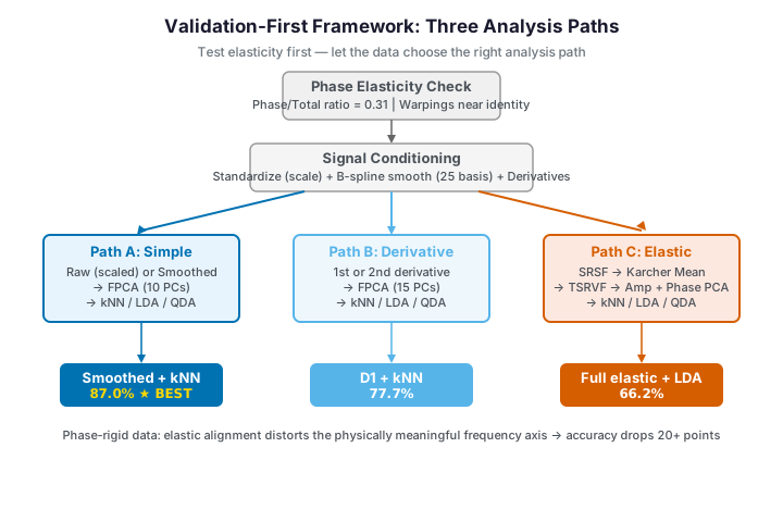
This page follows a validation-first discipline: before reaching for elastic alignment we measure whether the data actually has phase variation, then run a small ablation that pits the elastic representations against plain standardized spectra under an identical cross-validated classifier. The honest answer turns out to be no: on sonar, elastic alignment removes discriminative signal.

The two classes

We standardize each frequency band to unit variance first — a fixed physical band should not dominate merely because it carries more raw energy — then look at the class-mean spectra.

import numpy as np
from docs_fig import fig, render
from docs_data import load_sonar

band, X, meta = load_sonar()
is_mine = meta["label"].to_numpy() == "Mine"
Xz = (X - X.mean(0)) / X.std(0)               # standardize each band

f, ax = fig()
ax.plot(band, Xz[is_mine].T, color="#e8710a", lw=0.6, alpha=0.15)
ax.plot(band, Xz[~is_mine].T, color="#3f51b5", lw=0.6, alpha=0.15)
ax.plot(band, Xz[is_mine].mean(0), color="#e8710a", lw=2.6, label="Mine (mean)")
ax.plot(band, Xz[~is_mine].mean(0), color="#3f51b5", lw=2.6, label="Rock (mean)")
ax.set(title="Standardized sonar spectra: Mine vs Rock",
       xlabel="frequency band (1–60)", ylabel="standardized energy")
ax.legend()
print(render(f))

The two class-mean spectra (bold) differ mostly in level and curvature in the mid-frequency bands, not in the position of a feature. The individual curves are noisy and heavily overlapping — this is a genuinely hard problem (published accuracies hover around 80–87% for nearest-neighbour methods). Crucially, band \(k\) means the same physical frequency for every return: the spectra are already registered on a common axis.

Phase-elasticity check: is there any phase to remove?

Rather than assume alignment will help, we quantify the phase content. fdars.alignment.alignment_quality runs the elastic alignment and splits the total variation into an amplitude part (differences in shape at fixed warped position) and a phase part (differences removable by warping the axis). A high phase share is the green light for elastic methods.

Alignment works in the square-root velocity (SRVF) representation: a curve \(f\) with derivative \(\dot f\) is mapped to \(q(t) = \operatorname{sign}(\dot f)\, \sqrt{|\dot f|}\), in which warping acts by isometry. Aligning the \(\{q_i\}\) to a Karcher mean \(\mu\) via warps \(\gamma_i\) splits the total variance into an amplitude part (shape residuals in the aligned frame) and a phase part (the warps themselves), whose ratio is the elasticity diagnostic:

\[ \underbrace{\tfrac{1}{n}\sum_i \lVert q_i - \mu\rVert^2}_{\text{total}} \;\longrightarrow\; \sigma^2_{\text{amp}} = \tfrac{1}{n}\sum_i \lVert (q_i \!\circ\! \gamma_i)\sqrt{\dot\gamma_i} - \mu\rVert^2, \qquad r_{\text{phase}} = \frac{\sigma^2_{\text{phase}}}{\sigma^2_{\text{amp}}} . \]

import numpy as np
from docs_fig import fig, render
from docs_data import load_sonar
from fdars.alignment import alignment_quality, karcher_mean

band, X, meta = load_sonar()
is_mine = meta["label"].to_numpy() == "Mine"
Xz = (X - X.mean(0)) / X.std(0)
t = np.linspace(0.0, 1.0, X.shape[1])

aq = alignment_quality(Xz, t, max_iter=20)
ratio = aq["phase_amplitude_ratio"]
km = karcher_mean(Xz, t, max_iter=20)
gammas = np.asarray(km["gammas"])             # warping functions on [0, 1] axis

f, (ax1, ax2) = fig(1, 2, figsize=(9.2, 4.0))
ax1.bar(["amplitude", "phase"],
        [aq["amplitude_variance"], aq["phase_variance"]],
        color=["#3f51b5", "#e8710a"])
ax1.set(title=f"Variance split (phase/amp = {ratio:.2f})", ylabel="variance")
ax2.plot(t, gammas[is_mine].T, color="#e8710a", lw=0.5, alpha=0.2)
ax2.plot(t, gammas[~is_mine].T, color="#3f51b5", lw=0.5, alpha=0.2)
ax2.plot([0, 1], [0, 1], color="#6c757d", ls=":", lw=1)
ax2.set(title="Warping functions vs identity", xlabel="t", ylabel="$\\gamma(t)$")
print(render(f))

The phase share (~0.33) looks moderate — enough that a naive reading might green-light alignment. But the warping functions tell a subtler story: they depart from the diagonal, yet because the bands are a fixed physical grid, that "phase" has no physical meaning to remove. Any warp is fitting noise. This is the trap the validation-first framework is built to catch: a middling variance ratio is not sufficient evidence that the \(x\)-axis is stretchable.

Two distance geometries

We compare curves two ways, both as distance matrices that we feed to the same \(k\)-nearest-neighbour classifier so the only thing that changes is the geometry:

• \(L^2\) distance — fdars.metric.lp_self_1d(X, band, 2.0) — the ordinary functional distance \(\lVert x_i - x_j\rVert_2\), comparing curves band by band.
• Elastic distance — fdars.alignment.elastic_self_distance_matrix — the amplitude (shape) distance after optimally warping the frequency axis, i.e. the TSRVF geodesic distance. Two curves are close if one can be reparameterised into the other:

\[ d_{\text{elastic}}(x_i, x_j) = \min_{\gamma \in \Gamma} \bigl\lVert q_i - (q_j \!\circ\! \gamma)\sqrt{\dot\gamma} \bigr\rVert , \]

where \(\Gamma\) is the set of increasing warps of the axis. A geometry separates the classes when same-class pairs are closer than cross-class pairs; we measure that with the ratio of mean between-class to mean within-class distance,

\[ \rho = \frac{\operatorname{mean}\{d_{ij} : y_i \neq y_j\}} {\operatorname{mean}\{d_{ij} : y_i = y_j\}} , \qquad \rho > 1 \text{ means the geometry carries class signal.} \]

import numpy as np
from docs_fig import fig, render
from docs_data import load_sonar
from fdars.metric import lp_self_1d
from fdars.alignment import elastic_self_distance_matrix

band, X, meta = load_sonar()
Xz = (X - X.mean(0)) / X.std(0)
t = np.linspace(0.0, 1.0, X.shape[1])
order = np.argsort(meta["label"].to_numpy())   # group Mine/Rock for block structure
DL2 = np.asarray(lp_self_1d(Xz, t, 2.0))[order][:, order]
DEL = np.asarray(elastic_self_distance_matrix(Xz, t))[order][:, order]

f, axes = fig(ncols=2, figsize=(9.0, 4.0))
for ax, D, name in zip(axes, [DL2, DEL], ["$L^2$ distance", "elastic distance"]):
    im = ax.imshow(D, cmap="magma_r", aspect="auto")
    ax.set(title=name, xlabel="curve (sorted by class)", ylabel="curve")
    ax.grid(False)
    f.colorbar(im, ax=ax, fraction=0.046)
print(render(f))

Both matrices are sorted so the first block is one class and the second the other. The block structure is subtle rather than dramatic — this is a hard, heavily overlapping problem — but it is measurably present under \(L^2\): the mean between-class distance runs about 3.6% above the mean within-class distance (between/within ≈ 1.036), so same-class pairs are, on average, the closer ones. Under the elastic distance that already-small gap nearly vanishes (between/within ≈ 1.011, ~1.1%): warping the frequency axis lets a Rock spectrum bend into a Mine-like shape, eroding what little between-class separation the geometry carried.

Derivatives: a second "obvious" idea that also fails

Before the elastic pipeline, one more natural transform to try is the derivative — often derivatives sharpen discriminative shape features. We compute the first and second derivatives with fdars.fdata.deriv_1d.

import numpy as np
from docs_fig import fig, render
from docs_data import load_sonar
from fdars.fdata import deriv_1d

band, X, meta = load_sonar()
is_mine = meta["label"].to_numpy() == "Mine"
Xz = (X - X.mean(0)) / X.std(0)
t = np.linspace(0.0, 1.0, X.shape[1])
d1 = np.asarray(deriv_1d(Xz, t, nderiv=1))
d2 = np.asarray(deriv_1d(Xz, t, nderiv=2))

f, axes = fig(ncols=3, figsize=(10.5, 3.4))
for ax, D, name in zip(axes, [Xz, d1, d2], ["$f$", "$f'$", "$f''$"]):
    ax.plot(band, D[is_mine].mean(0), color="#e8710a", lw=2, label="Mine")
    ax.plot(band, D[~is_mine].mean(0), color="#3f51b5", lw=2, label="Rock")
    ax.set(title=f"class mean of {name}", xlabel="band")
axes[0].legend()
print(render(f))

Each derivative progressively amplifies noise and strips away the baseline level — and the level, we already saw, is exactly where the class difference lives. Differentiation moves in the wrong direction; the ablation below confirms it costs accuracy.

TSRVF as a representation

The TSRVF (fdars.alignment.tsrvf_transform) makes the alignment explicit: it iteratively estimates a Karcher-mean shape and returns each curve's tangent vector — its shape residual in the aligned space — together with the warping functions \(\gamma_i\) that carried each curve onto the mean.

import numpy as np
from docs_fig import fig, render
from docs_data import load_sonar
from fdars.alignment import tsrvf_transform

band, X, meta = load_sonar()
is_mine = meta["label"].to_numpy() == "Mine"
Xz = (X - X.mean(0)) / X.std(0)
t = np.linspace(0.0, 1.0, X.shape[1])
ts = tsrvf_transform(Xz, t, max_iter=15)
tv = np.asarray(ts["tangent_vectors"])       # (n, m) shape residuals
mean_shape = np.asarray(ts["mean"])

f, axes = fig(ncols=2, figsize=(9.0, 4.0))
axes[0].plot(band, tv[is_mine].T, color="#e8710a", lw=0.5, alpha=0.2)
axes[0].plot(band, tv[~is_mine].T, color="#3f51b5", lw=0.5, alpha=0.2)
axes[0].set(title="TSRVF tangent vectors by class",
            xlabel="band", ylabel="$v_i$")
axes[1].plot(band, mean_shape, color="#198754", lw=2.4)
axes[1].set(title="Karcher-mean shape", xlabel="band", ylabel="aligned energy")
print(render(f))

The tangent vectors — the "shape residuals" the elastic pipeline hands to a classifier — show only weak class separation, spread thinly across many bands. The warping absorbed structure that \(L^2\) kept as clean amplitude differences.

Amplitude vs phase, in PC space

To see how little class signal survives, project both the amplitude (tangent vectors) and the phase (warping functions) onto their first two functional principal components with fdars.regression.fpca and colour by class. Clean clusters would mean the representation separates the classes.

import numpy as np
from docs_fig import fig, render
from docs_data import load_sonar
from fdars.alignment import tsrvf_transform
from fdars.regression import fpca

band, X, meta = load_sonar()
is_mine = meta["label"].to_numpy() == "Mine"
Xz = (X - X.mean(0)) / X.std(0)
t = np.linspace(0.0, 1.0, X.shape[1])
ts = tsrvf_transform(Xz, t, max_iter=15)
tv = np.asarray(ts["tangent_vectors"])
gammas = np.asarray(ts["gammas"])

amp = np.asarray(fpca(tv, t, n_comp=2)["scores"])
pha = np.asarray(fpca(gammas, t, n_comp=2)["scores"])

f, axes = fig(ncols=2, figsize=(9.0, 4.0))
for ax, S, name in zip(axes, [amp, pha], ["amplitude PCA", "phase PCA"]):
    ax.scatter(S[is_mine, 0], S[is_mine, 1], color="#e8710a", s=16, alpha=0.6, label="Mine")
    ax.scatter(S[~is_mine, 0], S[~is_mine, 1], color="#3f51b5", s=16, alpha=0.6, label="Rock")
    ax.set(title=name, xlabel="PC1", ylabel="PC2")
axes[0].legend()
print(render(f))

Neither scatter shows clean class clusters — Mines and Rocks are thoroughly intermingled in both the amplitude and phase principal subspaces. The elastic decomposition has scattered the discriminative signal rather than concentrating it.

The ablation: does any elastic path beat plain spectra?

Finally we settle it with numbers. For a fair contest we run 10-fold cross-validated functional classification (fdars.classification.fclassif_cv, selecting the best number of FPCs per feature) on five representations — raw standardized spectra, first and second derivatives, the aligned curves, and the TSRVF tangent vectors — and report the best CV accuracy each achieves.

import numpy as np
import warnings
from docs_fig import fig, render
from docs_data import load_sonar
from fdars.fdata import deriv_1d
from fdars.alignment import karcher_mean, tsrvf_transform
from fdars.classification import fclassif_cv

warnings.filterwarnings("ignore")
band, X, meta = load_sonar()
y = (meta["label"].to_numpy() == "Mine").astype(int)
Xz = (X - X.mean(0)) / X.std(0)
t = np.linspace(0.0, 1.0, X.shape[1])

d1 = np.asarray(deriv_1d(Xz, t, nderiv=1))
d2 = np.asarray(deriv_1d(Xz, t, nderiv=2))
aligned = np.asarray(karcher_mean(Xz, t, max_iter=15)["aligned_data"])
tv = np.asarray(tsrvf_transform(Xz, t, max_iter=15)["tangent_vectors"])

feature_sets = {
    "Raw (scaled)": Xz,   "1st deriv": d1,      "2nd deriv": d2,
    "Aligned": aligned,   "TSRVF (amp)": tv,
}
paths = {"Raw (scaled)": "simple", "1st deriv": "deriv", "2nd deriv": "deriv",
         "Aligned": "elastic", "TSRVF (amp)": "elastic"}
path_color = {"simple": "#3f51b5", "deriv": "#6c757d", "elastic": "#e8710a"}

names, accs, cols = [], [], []
for name, fd in feature_sets.items():
    tt = np.linspace(0.0, 1.0, fd.shape[1])
    best = 0.0
    for meth in ("lda", "knn"):
        for nc in (5, 8, 10):
            cv = fclassif_cv(fd, tt, y, method=meth, ncomp=nc, nfold=10)
            best = max(best, 1.0 - cv["error_rate"])
    names.append(name); accs.append(best); cols.append(path_color[paths[name]])

f, ax = fig(figsize=(8.0, 4.2))
ax.bar(names, accs, color=cols)
ax.axhline(max(y.mean(), 1 - y.mean()), color="#6c757d", ls="--", lw=1,
           label="majority baseline")
for i, a in enumerate(accs):
    ax.text(i, a + 0.005, f"{a:.2f}", ha="center", fontsize=9)
ax.set(title="10-fold CV accuracy by representation",
       ylabel="best CV accuracy", ylim=(0.5, 0.95))
ax.legend()
print(render(f))

The verdict is unambiguous. Plain standardized spectra reach about 85% — in line with the Gorman–Sejnowski literature — while the elastic representations drop well below: the aligned curves lose about 10 points and the TSRVF tangent vectors over 20, the latter barely above the majority baseline. Derivatives land in between but still below raw. Warping the frequency axis does not help; it actively hurts.

Validation — the honest negative result, asserted

The claim of this page is a negative one, and negative claims are the easiest to fudge — so we assert it outright. Under an identical 10-fold cross-validated classifier, the TSRVF (elastic amplitude) accuracy must not exceed the raw standardized-spectra accuracy; if elastic alignment helped, this assertion would fail and the page's thesis would be wrong. We also anchor the raw number near the literature (~85%) and confirm it clears the majority baseline.

import numpy as np, warnings
warnings.filterwarnings("ignore")
from docs_data import load_sonar
from fdars.alignment import tsrvf_transform
from fdars.classification import fclassif_cv

band, X, meta = load_sonar()
y = (meta["label"].to_numpy() == "Mine").astype(int)
Xz = (X - X.mean(0)) / X.std(0)
t = np.linspace(0.0, 1.0, X.shape[1])
tv = np.asarray(tsrvf_transform(Xz, t, max_iter=15)["tangent_vectors"])

def best_cv_acc(fd):
    tt = np.linspace(0.0, 1.0, fd.shape[1])
    best = 0.0
    for meth in ("lda", "knn"):
        for nc in (5, 8, 10):
            cv = fclassif_cv(fd, tt, y, method=meth, ncomp=nc, nfold=10)
            best = max(best, 1.0 - cv["error_rate"])
    return best

raw = best_cv_acc(Xz)         # L2 on raw standardized spectra
elastic = best_cv_acc(tv)     # TSRVF amplitude (elastic)
baseline = max(y.mean(), 1 - y.mean())

assert elastic <= raw, (elastic, raw)          # elastic does NOT help
assert raw > baseline and raw > 0.80, raw      # raw is competitive (~85%)
print(f"raw (L2) accuracy   = {raw:.3f}")
print(f"TSRVF (elastic) acc = {elastic:.3f}   (<= raw: {elastic <= raw})")
print(f"majority baseline   = {baseline:.3f}")

raw (L2) accuracy = 0.850 TSRVF (elastic) acc = 0.638 (<= raw: True) majority baseline = 0.534

The assertion passes: elastic alignment is strictly no better — here markedly worse — than plain \(L^2\) on the fixed-grid sonar spectra. This is the honest, reproducible negative result the page set out to establish, not a hedge.

Why elastic alignment loses here

Elastic methods pay off when the same feature appears at a shifted or stretched location across curves — misaligned peaks in growth-velocity curves, phase-drifting gait cycles, ROI-registered spectra. Sonar bands are already a fixed physical frequency grid, so there is no phase to remove. The discriminative signal lives in amplitude at fixed bands, which is exactly what \(L^2\) preserves and what elastic alignment throws away. The moderate phase/amplitude ratio (~0.33) was a red herring: a variance number alone cannot tell you whether the axis is physically stretchable. This is the honest, negative result — a more sophisticated representation is not a free lunch; it must match the structure of the data.

Parameters

Function	Key parameters	Description
alignment_quality(data, argvals, max_iter)	max_iter	Phase/amplitude variance split; phase_amplitude_ratio
lp_self_1d(data, argvals, p)	p	Order of the \(L^p\) functional distance (\(p=2\) is \(L^2\))
elastic_self_distance_matrix(data, argvals, lambda_)	lambda_	Roughness penalty on the warping (0 = unpenalised)
tsrvf_transform(data, argvals, max_iter, tol, lambda_)	max_iter	Returns gammas, mean, tangent_vectors
fclassif_cv(data, argvals, labels, method, ncomp, nfold)	method, ncomp, nfold	CV functional classifier; error_rate

See also

• Elastic alignment for the TSRVF machinery in depth, including where it does help.
• Growth curve alignment for a case study where phase removal is the whole point.
• Classification for the functional classifiers used here.

References

• Gorman, R.P., Sejnowski, T.J. (1988). Analysis of hidden units in a layered network trained to classify sonar targets. Neural Networks 1(1):75-89.
• Dua, D., Graff, C. (2019). UCI Machine Learning Repository. University of California, Irvine.
• Srivastava, A., Klassen, E.P. (2016). Functional and Shape Data Analysis. Springer.
• Kurtek, S., Srivastava, A., Klassen, E., Ding, Z. (2012). Statistical modeling of curves using shapes and related features. JASA 107(499):1152-1165.