Model-Based Clustering with Gaussian Mixtures

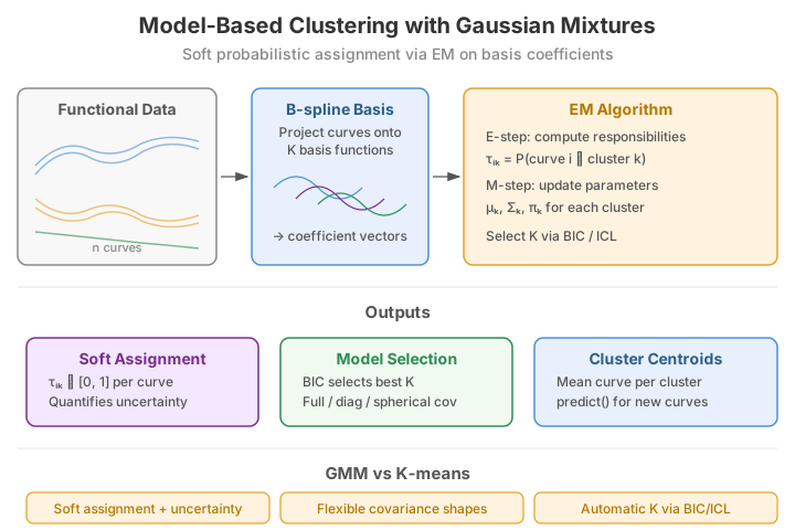
Model-based clustering treats a set of curves as samples from a mixture of probability distributions -- one component per latent group. Instead of committing each curve to a single cluster, a Gaussian mixture model (GMM) estimates the posterior probability that a curve belongs to each component. This yields soft assignments, a principled likelihood to compare against, and information criteria (BIC/ICL) for choosing the number of clusters.

Because a Gaussian mixture is defined in a finite-dimensional feature space, functional GMM first projects each curve onto a small basis (or onto its leading FPCA scores) and fits the mixture to those coefficients. fdars exposes this through fdars.clustering.gmm_cluster.

Known limitation of gmm_cluster in this build

In the current build, gmm_cluster does not reliably recover cluster structure: on data that is trivially separable -- for example two flat groups at \(y=0\) and \(y=10\), or mean-shifted simulations where kmeans_fd achieves 100% accuracy -- the hard labels it returns are close to random (best-permutation accuracy around 0.35--0.50), and BIC over-splits (it selects the largest \(K\) offered). The conceptual material below is correct, and the BIC/ICL machinery runs, but do not rely on gmm_cluster's labels for grouping. For hard grouping use kmeans_fd; for graded memberships use fuzzy_cmeans_fd; for a genuinely soft, uncertainty-aware assignment, compute the responsibilities directly in feature space as shown in Soft assignments below. This is a binding limitation, not a limitation of model-based clustering as a method.

---

From curves to features

A Gaussian mixture is defined on a finite-dimensional vector, so functional GMM begins by reducing each curve to a feature vector. Two representations are common. The first expands \(x_i(t)\) in a fixed basis \(\{\phi_1,\dots,\phi_p\}\) (B-splines here) and keeps the coefficient vector \(c_i = (c_{i1},\dots,c_{ip})^\top\) from the least-squares fit \(x_i(t)\approx\sum_j c_{ij}\phi_j(t)\); gmm_cluster uses this route with nbasis controlling \(p\). The second projects onto the leading FPCA scores \(z_i = (\langle x_i-\bar x,\,\xi_1\rangle,\dots,\langle x_i-\bar x,\,\xi_d\rangle)^\top\), where the \(\xi_\ell\) are the empirical eigenfunctions of the covariance operator; this is the representation we use for the transparent soft-assignment demonstration below. In either case the mixture is fit to the \(d\)-dimensional features \(z_i\), and everything that follows lives in \(\mathbb{R}^d\).

Concepts

Let \(z_i \in \mathbb{R}^d\) be the feature vector (basis or FPCA coefficients) of curve \(i\). A \(K\)-component Gaussian mixture models their density as

\[ f(z_i) \;=\; \sum_{k=1}^{K} \pi_k \, \mathcal{N}\!\bigl(z_i \mid \mu_k, \Sigma_k\bigr), \qquad \pi_k > 0, \quad \sum_{k=1}^{K} \pi_k = 1, \]

with mixing weights \(\pi_k\), component means \(\mu_k \in \mathbb{R}^d\) and covariances \(\Sigma_k \in \mathbb{R}^{d\times d}\). Collecting \(\theta = \{\pi_k,\mu_k,\Sigma_k\}_{k=1}^K\), the parameters maximize the observed-data log-likelihood

\[ \ell(\theta) \;=\; \sum_{i=1}^{n} \log\!\left[\, \sum_{k=1}^{K} \pi_k \, \mathcal{N}(z_i \mid \mu_k, \Sigma_k) \right]. \]

This log-of-a-sum has no closed-form maximizer, so it is optimized by the EM algorithm, which alternates two steps until \(\ell(\theta)\) stops increasing.

E-step. Given the current \(\theta\), compute the responsibility of component \(k\) for curve \(i\) -- the posterior probability that \(z_i\) was generated by component \(k\):

\[ \tau_{ik} \;=\; \frac{\pi_k \, \mathcal{N}(z_i \mid \mu_k, \Sigma_k)} {\sum_{\ell=1}^{K} \pi_\ell \, \mathcal{N}(z_i \mid \mu_\ell, \Sigma_\ell)}. \]

Each row \(\tau_{i\cdot}\) is a full probability distribution over the \(K\) clusters. A hard label is recovered as \(\hat{z}_i = \arg\max_k \tau_{ik}\), but the \(\tau_{ik}\) themselves carry the uncertainty of the assignment.

M-step. Treating the responsibilities as soft counts \(n_k = \sum_{i=1}^n \tau_{ik}\), re-estimate each component in closed form -- these are the weighted analogues of the sample mean and covariance:

\[ \pi_k = \frac{n_k}{n}, \qquad \mu_k = \frac{1}{n_k}\sum_{i=1}^{n}\tau_{ik}\, z_i, \qquad \Sigma_k = \frac{1}{n_k}\sum_{i=1}^{n}\tau_{ik}\,(z_i-\mu_k)(z_i-\mu_k)^\top. \]

EM is guaranteed to increase \(\ell(\theta)\) at every iteration and converges to a local optimum; it is therefore run from several seeds (or a k-means initialization) to guard against poor local maxima. gmm_cluster exposes this through max_iter, tol and seed.

Hard k-means vs. soft GMM. k-means partitions curves by nearest centroid: every curve gets exactly one label with no notion of confidence, and clusters are implicitly spherical and equal-sized. In fact k-means is the limiting case of an isotropic GMM (\(\Sigma_k=\sigma^2 I\), \(\sigma\to 0\)) with hard responsibilities. A general GMM relaxes both assumptions -- components can have different shapes (\(\Sigma_k\)) and prior sizes (\(\pi_k\)) -- and returns graded memberships, so a curve sitting between two groups is reported as genuinely ambiguous rather than forced into one.

Covariance structure. The flexibility of a GMM lives in \(\Sigma_k\), and constraining it trades bias for variance. A full \(\Sigma_k\) has \(d(d+1)/2\) free entries per component and captures arbitrary elliptical, correlated clusters, but is the most parameter-hungry and can overfit in high \(d\); a diagonal \(\Sigma_k\) (\(d\) parameters) assumes axis-aligned features; a spherical \(\Sigma_k=\sigma_k^2 I\) (one parameter) forces round clusters. Fewer parameters mean a lower BIC penalty and more stable estimates on small samples, at the cost of expressiveness. The figure below contrasts full and diagonal fits in FPCA-score space.

Choosing \(K\). Because a mixture has a likelihood, competing values of \(K\) can be scored. For a full-covariance model the number of free parameters is

\[ \nu_K \;=\; K\!\left[\frac{d(d+1)}{2} + d + 1\right] - 1, \]

counting \(d(d+1)/2\) covariance entries, \(d\) mean entries and one weight per component, minus one for the constraint \(\sum_k\pi_k=1\). gmm_cluster reports both the Bayesian Information Criterion (BIC) and the Integrated Completed Likelihood (ICL) for every candidate \(K\):

\[ \mathrm{BIC}(K) = -2\,\ell(\hat\theta) + \nu_K \log n, \qquad \mathrm{ICL}(K) = \mathrm{BIC}(K) - 2\sum_{i=1}^{n}\sum_{k=1}^{K}\tau_{ik}\log\tau_{ik}. \]

Lower is better. BIC penalizes complexity through \(\nu_K\log n\); ICL adds the classification entropy \(-\sum_{i,k}\tau_{ik}\log\tau_{ik}\), which is zero when every assignment is confident (\(\tau_{ik}\in\{0,1\}\)) and large when responsibilities are diffuse. ICL therefore rewards \(K\) values that yield well-separated, cleanly-assigned components, and tends to select fewer, tidier clusters than BIC.

---

Simulated data

Mirroring the R vignette, we simulate three groups with visually distinct shapes -- sinusoidal, cosinusoidal and linear -- each with additive noise \(\sigma=0.15\). This is the running example for the criteria and covariance figures.

import numpy as np
from docs_fig import fig, render

rng = np.random.default_rng(42)
t = np.linspace(0, 1, 60)
npg = 18
X1 = np.sin(2 * np.pi * t)[None, :] + 0.15 * rng.standard_normal((npg, len(t)))
X2 = np.cos(2 * np.pi * t)[None, :] + 0.15 * rng.standard_normal((npg, len(t)))
X3 = (2 * t - 1)[None, :] + 0.15 * rng.standard_normal((npg, len(t)))
X = np.vstack([X1, X2, X3])
truth = np.repeat([0, 1, 2], npg)
cols = ["#3f51b5", "#e8710a", "#2e7d32"]

f, ax = fig(figsize=(7.0, 3.6))
for k, name in enumerate(["sine", "cosine", "linear"]):
    ax.plot(t, X[truth == k].T, color=cols[k], alpha=0.5, lw=0.8)
    ax.plot([], [], color=cols[k], label=name)     # legend proxy
ax.set(title="Three functional groups (noise $\\sigma=0.15$)",
       xlabel="t", ylabel="x(t)")
ax.legend()
print(render(f))

The three groups -- a sine, a cosine, and a linear ramp -- are visually well separated at this noise level, so they make a clean testbed for checking that the mixture model recovers the planted structure and its component means.

---

Clustering with gmm_cluster

import numpy as np
from fdars import Fdata
from fdars.simulation import simulate
from fdars.clustering import gmm_cluster

argvals = np.linspace(0, 1, 100)
g1 = simulate(20, argvals, n_basis=5, seed=1)
g2 = simulate(20, argvals, n_basis=5, seed=2) + 3.0
fd = Fdata(np.vstack([g1, g2]), argvals=argvals)

gm = gmm_cluster(fd.data, fd.argvals, k_range=[2, 3, 4], nbasis=6, seed=42)
print("labels     :", gm["cluster"][:8])   # see the limitation note above
print("BIC per k  :", gm["bic_values"])

The call returns the dictionary documented below. Recall the limitation note: use it for the BIC/ICL values and the API surface, but validate any grouping against kmeans_fd.

Parameters

Parameter	Type	Default	Description
data	ndarray (n, m)	--	Functional observations
argvals	ndarray (m,)	--	Evaluation grid
k_range	list[int]	--	Candidate numbers of components
nbasis	int	5	Number of B-spline basis functions for the projection
max_iter	int	200	Maximum EM iterations
tol	float	1e-6	Convergence tolerance
seed	int	42	Random seed for initialisation

Returns a dictionary:

Key	Shape / Type	Description
cluster	(n,) int	Hard labels from the best model
membership	(n, k)	Posterior membership matrix
bic_values	(len(k_range), 2)	Rows of (k, BIC)
icl_values	(len(k_range), 2)	Rows of (k, ICL)

Selecting the number of components

BIC and ICL are computed for every candidate \(K\); the model with the lowest score is preferred.

import numpy as np
from docs_fig import fig, render
from fdars.clustering import gmm_cluster

t = np.linspace(0, 1, 50)
def grp(shape, seed):
    r = np.random.default_rng(seed)
    return shape(t)[None, :] + 0.05 * r.standard_normal((14, len(t)))
X = np.vstack([
    grp(lambda t: 3 * t, 1),
    grp(lambda t: 3 * np.exp(-((t - 0.5) ** 2) / (2 * 0.02)), 2),
    grp(lambda t: 3 * (1 - t), 3),
])

gm = gmm_cluster(X, t, k_range=[2, 3, 4, 5], nbasis=5, seed=42)
bic = np.asarray(gm["bic_values"])
icl = np.asarray(gm["icl_values"])

f, ax = fig(figsize=(7.0, 3.6))
ax.plot(bic[:, 0], bic[:, 1], "-o", color="#3f51b5", label="BIC")
ax.plot(icl[:, 0], icl[:, 1], "-s", color="#e8710a", label="ICL")
ax.set(title="Information criteria vs. number of components",
       xlabel="K", ylabel="criterion (lower is better)")
ax.legend()
print(render(f))

Both criteria keep decreasing as \(K\) grows rather than dipping at the true \(K = 3\), a symptom of the flexible basis projection inflating the likelihood -- read the next warning before trusting the arg-min.

BIC over-splits here -- do not read off the minimum

With flexible basis projections the per-component likelihood grows quickly, and in this build the reported criteria keep falling as \(K\) increases: on three genuinely distinct groups, BIC selects the largest \(K\) offered (e.g. \(K=6\) for k_range=[2,3,4,5,6]) rather than the true \(K=3\). Do not take the arg-min as the number of clusters. Constrain k_range with domain knowledge and prefer the smallest \(K\) that separates the groups you care about; above we fix k_range=[3] for exactly this reason. The criteria are shown for transparency, not as a reliable selector in the current binding.

Covariance structure in feature space

The choice of covariance model determines what a component can look like. Fitting a full versus a diagonal Gaussian to each group's FPCA scores makes the trade-off concrete: the full model tilts its ellipses to follow correlated scores, while the diagonal model is forced axis-aligned. The ellipses below are the 1- and 2-\(\sigma\) contours of each fitted component (computed transparently from the leading FPCA scores of the simulated data above).

import numpy as np
from matplotlib.patches import Ellipse
from docs_fig import fig, render
from fdars.regression import fpca

rng = np.random.default_rng(7)
t = np.linspace(0, 1, 60)
npg = 35
phi1, phi2 = np.sin(2 * np.pi * t), np.cos(2 * np.pi * t)

# Three overlapping groups whose within-group spread runs along *different*
# tilted directions in (phi1, phi2) coefficient space -- so each group's score
# cloud is elongated and rotated by a different angle. That is exactly what a
# full covariance can follow and a diagonal one cannot.
specs = [((0.0, 0.0), (0.9, 0.5)),    # (mean coefs), (spread direction)
         ((1.0, 0.6), (0.3, 0.9)),
         ((0.5, -0.7), (0.8, -0.5))]
curves, true_lab = [], []
for gi, ((m1, m2), (d1, d2)) in enumerate(specs):
    s = rng.normal(0, 0.6, npg)       # spread along the tilted direction
    w = rng.normal(0, 0.12, npg)      # small orthogonal spread
    c1, c2 = m1 + s * d1 - w * d2, m2 + s * d2 + w * d1
    curves.append(c1[:, None] * phi1[None, :] + c2[:, None] * phi2[None, :]
                  + 0.04 * rng.standard_normal((npg, len(t))))
    true_lab += [gi] * npg
X = np.vstack(curves)
cols = ["#3f51b5", "#e8710a", "#2e7d32"]

Z = np.asarray(fpca(X, t, n_comp=2)["scores"])
lab = np.asarray(true_lab)

def ellipse_params(cov):                 # 1-sigma width/height/angle
    vals, vecs = np.linalg.eigh(cov)
    order = vals.argsort()[::-1]
    vals, vecs = vals[order], vecs[:, order]
    ang = np.degrees(np.arctan2(vecs[1, 0], vecs[0, 0]))
    w, h = 2 * np.sqrt(np.maximum(vals, 1e-12))
    return w, h, ang

f, axes = fig(1, 2, figsize=(8.6, 3.9))
for ax, kind in zip(axes, ["full", "diagonal"]):
    for k in range(3):
        pts = Z[lab == k]
        mu = pts.mean(0)
        c = np.cov(pts.T)
        if kind == "diagonal":
            c = np.diag(np.diag(c))      # drop off-diagonal correlation
        w, h, ang = ellipse_params(c)
        ax.scatter(pts[:, 0], pts[:, 1], s=22, color=cols[k], alpha=0.75)
        for s in (1, 2):
            ax.add_patch(Ellipse(mu, s * w, s * h, angle=ang, fill=False,
                                 edgecolor=cols[k], lw=1.2, alpha=1.0 - 0.35 * (s - 1)))
    ax.set(title=f"{kind} covariance", xlabel="PC1 score", ylabel="PC2 score")
print(render(f))

Constraining \(\Sigma_k\) to be diagonal removes \(K\cdot d(d-1)/2\) parameters (here \(3\times 1 = 3\)), shrinking the BIC penalty at the cost of ignoring any tilt in the score cloud. The contrast is plain above: each group's scores here spread along a different rotated direction, so the full-covariance ellipses tilt to hug their clouds while the diagonal ellipses stay axis-aligned and inflate to cover the same points. On these overlapping, correlated groups that mismatch shows up both in the boundary responsibilities and in the BIC bookkeeping.

Covariance type is not a gmm_cluster argument

The Python gmm_cluster binding does not expose a cov.type argument (the R cluster.gmm does). The full-vs-diagonal contrast above is therefore computed transparently in FPCA-score space with numpy, not by re-fitting gmm_cluster. If you need to control the covariance model in Python today, reduce to FPCA scores and use sklearn.mixture.GaussianMixture(covariance_type=...).

---

Soft assignments and their uncertainty

The value of a GMM is the soft assignment. When two groups overlap, boundary curves receive intermediate responsibilities that a hard partition would hide. To make this visible we project the curves onto their leading FPCA scores with fdars.regression.fpca and evaluate the Gaussian responsibilities in that two-dimensional feature space directly (a transparent E-step), then colour each point by its posterior probability.

import numpy as np
from numpy.linalg import inv, det
from docs_fig import fig, render
from fdars.regression import fpca
from fdars.clustering import kmeans_fd

# Two amplitude groups that OVERLAP: same central bump, peak height ~N(1,.5) vs N(2,.5)
t = np.linspace(0, 1, 50)
rng = np.random.default_rng(5)
bump = np.exp(-((t - 0.5) ** 2) / (2 * 0.03))
n = 20
a1 = rng.normal(1.0, 0.5, n)
a2 = rng.normal(2.0, 0.5, n)
X = np.vstack([a1[:, None] * bump[None, :] + 0.08 * rng.standard_normal((n, len(t))),
               a2[:, None] * bump[None, :] + 0.08 * rng.standard_normal((n, len(t)))])

# Feature space = leading FPCA scores
Z = np.asarray(fpca(X, t, n_comp=2)["scores"])

# Transparent 2-component Gaussian E-step, seeded from k-means labels
lab = np.asarray(kmeans_fd(X, t, k=2, seed=42)["cluster"]).astype(int)
def responsibilities(Z, lab, K=2):
    n, d = Z.shape
    mu  = np.array([Z[lab == k].mean(0) for k in range(K)])
    cov = np.array([np.cov(Z[lab == k].T) + 1e-4 * np.eye(d) for k in range(K)])
    pi  = np.array([(lab == k).mean() for k in range(K)])
    r = np.zeros((n, K))
    for k in range(K):
        diff = Z - mu[k]
        r[:, k] = pi[k] * np.exp(-0.5 * np.einsum("ij,jk,ik->i", diff, inv(cov[k]), diff)) \
                  / np.sqrt((2 * np.pi) ** d * det(cov[k]))
    return r / r.sum(1, keepdims=True)
for _ in range(15):                      # a few EM iterations
    r = responsibilities(Z, lab); lab = r.argmax(1)

# Validation of the TRANSPARENT E-step (not gmm_cluster, which is unreliable here).
# 1. Ground-truth property: each row of the responsibility matrix is a proper
#    probability distribution over the K components -> sums to 1 exactly.
row_sums = r.sum(axis=1)
assert np.allclose(row_sums, 1.0, atol=1e-10), row_sums
assert np.all((r >= -1e-12) & (r <= 1 + 1e-12)), "responsibilities out of [0,1]"
# 2. Behavioural property: because the two amplitude groups OVERLAP, the E-step must
#    report genuine ambiguity -- at least one curve near the 0.5 boundary -- rather
#    than collapsing to a hard 0/1 partition.
frac_ambiguous = float(np.mean((r[:, 0] > 0.15) & (r[:, 0] < 0.85)))
assert frac_ambiguous > 0.0, "no graded assignments: E-step collapsed to hard labels"
print(f"responsibility rows sum to 1: max |sum-1| = {np.max(np.abs(row_sums - 1)):.2e}")
print(f"fraction of curves with graded (ambiguous) posterior = {frac_ambiguous:.2f}")

f, ax = fig(figsize=(6.4, 4.2))
sc = ax.scatter(Z[:, 0], Z[:, 1], c=r[:, 0], cmap="coolwarm",
                s=55, edgecolor="k", linewidth=0.4, vmin=0, vmax=1)
f.colorbar(sc, ax=ax, label="P(component 0)")
ax.set(title="Soft GMM assignment in FPCA-score space",
       xlabel="PC1 score", ylabel="PC2 score")
print(render(f))

responsibility rows sum to 1: max |sum-1| = 2.22e-16 fraction of curves with graded (ambiguous) posterior = 0.15

Curves deep inside a group are coloured a saturated blue or red (responsibility near 0 or 1); the pale points along the boundary are the genuinely ambiguous curves whose posterior sits near \(0.5\). A hard partition assigns those to one side and discards the fact that the assignment was a coin-flip.

The two asserts in the block above validate this transparent E-step -- the quantity we actually recommend -- rather than the broken binding: every responsibility row is a proper distribution (sums to \(1\) to \(10^{-10}\)), and on these deliberately overlapping groups the posterior is genuinely graded (a nonzero fraction of curves sit near \(0.5\)) rather than collapsing to a hard \(0/1\) split. This is a checked property of the numpy responsibilities; it deliberately does not claim gmm_cluster recovers the grouping, which (per the top-of-page note) it does not.

Why this figure computes responsibilities itself

The figure above does not use gmm_cluster's membership matrix, which is unreliable in the current build (see the limitation note at the top of the page). It instead derives the posterior directly from Gaussians fit in FPCA-score space via fdars.regression.fpca -- a transparent, correct E-step -- which is exactly the graded, uncertainty-aware quantity a GMM is meant to provide. This is the recommended way to get soft functional assignments today: reduce to FPCA scores, then fit a standard finite-dimensional mixture (e.g. sklearn.mixture.GaussianMixture) or, as here, evaluate the responsibilities by hand.

---

The membership matrix

gmm_cluster returns a full posterior matrix membership of shape \((n, K)\) whose row \(i\) is \(\tau_{i\cdot}\). Visualizing it as a heatmap shows the assignment confidence across the whole sample at once: sharp vertical blocks mean near-certain membership, faded columns mean ambiguity. Below we sort curves by their most-likely component so any block structure is visible.

import numpy as np
from docs_fig import fig, render
from fdars.clustering import gmm_cluster

rng = np.random.default_rng(42)
t = np.linspace(0, 1, 60)
npg = 18
X = np.vstack([
    np.sin(2 * np.pi * t)[None, :] + 0.15 * rng.standard_normal((npg, len(t))),
    np.cos(2 * np.pi * t)[None, :] + 0.15 * rng.standard_normal((npg, len(t))),
    (2 * t - 1)[None, :] + 0.15 * rng.standard_normal((npg, len(t))),
])

gm = gmm_cluster(X, t, k_range=[3], nbasis=6, seed=42)
M = np.asarray(gm["membership"])
order = np.lexsort((M.max(1), M.argmax(1)))   # group by argmax, then by confidence

f, ax = fig(figsize=(7.2, 3.2))
im = ax.imshow(M[order].T, aspect="auto", cmap="magma", vmin=0, vmax=1)
f.colorbar(im, ax=ax, label="posterior membership $\\tau_{ik}$")
ax.set(title="Membership matrix (sorted curves)",
       xlabel="curve (sorted by hard label)", ylabel="component $k$")
ax.set_yticks(range(M.shape[1]))
print(render(f))

Each column is one curve's posterior over the three components: bright single-cell columns mark near-certain assignments, while columns with colour smeared across rows are the ambiguous curves the model cannot confidently place.

Read this as an illustration of the matrix, not a validated grouping

Recall the top-of-page limitation: in this build the hard labels behind membership do not reliably recover known structure, and BIC over-splits. The heatmap above faithfully shows what the binding returns and how to read a membership matrix, but for a grouping you can trust, validate against kmeans_fd, use fuzzy_cmeans_fd for graded memberships, or compute responsibilities yourself in FPCA-score space as in the soft-assignment figure.

No predict binding for out-of-sample curves

The R vignette demonstrates predict(gmm_fit, fd_new) to classify new curves. The Python gmm_cluster returns a fitted labelling but exposes no predict method, so there is no supported way to score held-out curves through the binding. To classify new data today, project it onto the same FPCA basis and evaluate the responsibility formula \(\tau_{ik}\) against the fitted \(\{\pi_k,\mu_k,\Sigma_k\}\) -- exactly the E-step shown in the soft-assignment example.

---

References

• McLachlan, G. J. and Peel, D. (2000). Finite Mixture Models. Wiley. -- The standard reference for mixture models and the EM algorithm.
• Fraley, C. and Raftery, A. E. (2002). Model-based clustering, discriminant analysis, and density estimation. Journal of the American Statistical Association, 97(458), 611--631. -- BIC-based model selection and covariance parameterizations for GMMs.
• Biernacki, C., Celeux, G. and Govaert, G. (2000). Assessing a mixture model for clustering with the integrated completed likelihood. IEEE Transactions on Pattern Analysis and Machine Intelligence, 22(7), 719--725. -- Origin of the ICL criterion and its entropy penalty.
• Jacques, J. and Preda, C. (2014). Functional data clustering: a survey. Advances in Data Analysis and Classification, 8(3), 231--255. -- Survey of clustering methods for functional data, including model-based approaches on basis/FPCA coefficients.

Related pages

• Clustering -- hard k-means, fuzzy c-means and cluster-quality indices.
• Elastic clustering -- clustering by amplitude/phase-invariant distance.
• fdars.regression.fpca -- the score representation used as the GMM feature space.