Scalar-on-Shape Regression

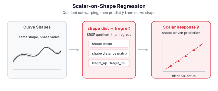
Ordinary scalar-on-function regression predicts a scalar response from the amplitude of a curve — its value at each fixed \(t\). But sometimes the response depends on the curve's shape: the geometric pattern of peaks and troughs, independent of how the curve is stretched or shifted along the \(t\)-axis. Two curves that are warped versions of one another have the same shape and, for a shape-driven response, should predict the same value.

Scalar-on-shape regression handles exactly this. We first quotient out warping with the elastic (SRSF) machinery in fdars.alignment, then regress the response on either a shape distance matrix (nonparametric) or shape principal-component scores (linear). This page builds both pipelines on a seeded example.

No single scalar_on_shape binding

The R package ships a purpose-built scalar.on.shape() estimator that jointly fits alignment and a penalised coefficient index. fdars for Python does not expose that one function; instead we compose the same idea from the shape primitives (shape_mean, shape_self_distance_matrix) plus the standard regressors. The results below are honest: the shape pipelines are competitive with, and often better than, naïve FPC regression on phase-variable data, but the margins depend on the problem.

import numpy as np
from scipy.stats import beta as beta_dist
from docs_fig import fig, render
from fdars.alignment import shape_mean

def make_shape_data(seed, n=60, m=60):
    """Curves = phase-warped copies of a shape whose amplitude drives y."""
    rng = np.random.default_rng(seed)
    t = np.linspace(0, 1, m)
    X = np.zeros((n, m)); y = np.zeros(n)
    for i in range(n):
        amp = rng.normal(0, 1)                              # shape signal
        base = amp * np.sin(2 * np.pi * t) + 0.4 * np.sin(4 * np.pi * t)
        a, b = rng.uniform(0.3, 3.0, size=2)               # phase nuisance
        gamma = beta_dist.cdf(t, a, b)
        X[i] = np.interp(gamma, t, base) + 0.05 * rng.standard_normal(m)
        y[i] = 2 * amp + rng.normal(0, 0.3)                # response from shape
    return t, X, y

t, X, y = make_shape_data(seed=3)
sm = shape_mean(X, t)
mean = np.asarray(sm["mean"])
aligned = np.asarray(sm["aligned_data"])

f, (a0, a1) = fig(1, 2, figsize=(11, 4))
a0.plot(t, X[:20].T, color="#3f51b5", lw=0.8, alpha=0.4)
a0.set(title="Raw curves (phase-warped)", xlabel="t", ylabel="X(t)")
a1.plot(t, aligned.T, color="#198754", lw=0.8, alpha=0.4)
a1.plot(t, mean, color="#e8710a", lw=2.6, label="shape mean")
a1.set(title="After alignment to the shape mean", xlabel="t", ylabel="X(t)")
a1.legend()
print(render(f))

The raw panel is a tangle of peaks at different \(t\)-locations — pure phase noise — while the aligned panel collapses them onto a common shape around the orange mean, exposing the amplitude variation that actually drives the response.

Concepts

A functional observation \(x(t)\) splits into an amplitude component (the shape of the curve) and a phase component (a warping \(\gamma\) of the \(t\)-axis). Two curves \(x_1, x_2\) share a shape when there is a warping \(\gamma\) with \(x_1 \approx x_2 \circ \gamma\). The elastic (Fisher–Rao) framework makes this precise through the square-root velocity function (SRVF); the resulting shape distance

\[ d_{\text{shape}}(x_1, x_2) = \min_{\gamma}\; \big\lVert q_1 - (q_2 \circ \gamma)\sqrt{\dot\gamma}\big\rVert_2 \]

is invariant to warping. The scalar-on-shape model then assumes the response depends on the curve only through its shape:

\[ y_i = g\!\left(\text{shape}(x_i)\right) + \varepsilon_i . \]

We estimate \(g\) in two ways. (1) Distance-based (nonparametric): feed the pairwise shape-distance matrix into the Nadaraya–Watson kernel regressor fregre_np, letting similar-shaped curves borrow strength. (2) Shape-PC (linear): align all curves to the shape mean, run FPCA on the aligned curves to obtain warping-invariant shape scores, and regress the response on those scores with fregre_lm.

Building the data

The predictor curves are phase-warped copies of a base shape whose amplitude carries the signal; the response depends on that amplitude, not on the warping. This is the regime where removing phase should help.

import numpy as np
from scipy.stats import beta as beta_dist

def make_shape_data(seed, n=60, m=60):
    rng = np.random.default_rng(seed)
    t = np.linspace(0, 1, m)
    X = np.zeros((n, m)); y = np.zeros(n)
    for i in range(n):
        amp = rng.normal(0, 1)                              # shape signal
        base = amp * np.sin(2 * np.pi * t) + 0.4 * np.sin(4 * np.pi * t)
        a, b = rng.uniform(0.3, 3.0, size=2)               # phase nuisance
        gamma = beta_dist.cdf(t, a, b)
        X[i] = np.interp(gamma, t, base) + 0.05 * rng.standard_normal(m)
        y[i] = 2 * amp + rng.normal(0, 0.3)
    return t, X, y

t, X, y = make_shape_data(seed=3)

Pipeline 1 — distance-based shape regression

shape_self_distance_matrix computes the full \(n \times n\) matrix of pairwise shape distances. Passing it to fregre_np gives a kernel regression whose geometry is defined by shape similarity, not pointwise amplitude.

import numpy as np
from fdars.alignment import shape_self_distance_matrix
from fdars.regression import fregre_np

D = np.asarray(shape_self_distance_matrix(X, t))   # (n, n) shape distances
np_fit = fregre_np(D, y, h=0.0)                    # h=0 -> automatic bandwidth

print(f"shape-NP R²:        {np_fit['r_squared']:.3f}")
print(f"selected bandwidth: {np_fit['h_func']:.3f}")

Function	Signature	Returns
shape_self_distance_matrix	(data, argvals, quotient="reparameterization", lambda_=0.0)	ndarray (n, n)
fregre_np	(dist_matrix, response, h=0.0)	dict: fitted_values, residuals, h_func, r_squared

The kernel regressor sees only this distance matrix, so it is worth looking at. Sorting rows and columns by the response \(y\) reveals whether shape-similar curves (small distances, dark cells) also share similar responses — the structure the kernel exploits:

import numpy as np
from scipy.stats import beta as beta_dist
from docs_fig import fig, render
from fdars.alignment import shape_self_distance_matrix

def make_shape_data(seed, n=60, m=60):
    rng = np.random.default_rng(seed)
    t = np.linspace(0, 1, m)
    X = np.zeros((n, m)); y = np.zeros(n)
    for i in range(n):
        amp = rng.normal(0, 1)
        base = amp * np.sin(2 * np.pi * t) + 0.4 * np.sin(4 * np.pi * t)
        a, b = rng.uniform(0.3, 3.0, size=2)
        gamma = beta_dist.cdf(t, a, b)
        X[i] = np.interp(gamma, t, base) + 0.05 * rng.standard_normal(m)
        y[i] = 2 * amp + rng.normal(0, 0.3)
    return t, X, y

t, X, y = make_shape_data(seed=3)
D = np.asarray(shape_self_distance_matrix(X, t))
order = np.argsort(y)                     # sort by response
Ds = D[np.ix_(order, order)]

f, ax = fig()
im = ax.imshow(Ds, cmap="viridis", origin="lower")
ax.set(title="Shape-distance matrix (rows/cols sorted by y)",
       xlabel="curve (by y rank)", ylabel="curve (by y rank)")
f.colorbar(im, ax=ax, label="shape distance")
print(render(f))

The dark block along the diagonal shows that curves with similar responses are also close in shape distance — a checkerboard would instead signal that shape carries no response information, and the kernel regressor would then fail.

Pipeline 2 — shape-PC linear regression

Aligning to the shape mean removes phase variation; FPCA on the aligned curves then yields shape scores. Regressing the response on these scores with fregre_lm gives an interpretable linear model whose coefficient function lives in the shape space.

import numpy as np
from fdars.alignment import shape_mean
from fdars.regression import fregre_lm

sm = shape_mean(X, t)
aligned = np.asarray(sm["aligned_data"])          # phase removed

lm_fit = fregre_lm(aligned, y, n_comp=6)          # FPC regression on shape
print(f"shape-PC R²: {lm_fit['r_squared']:.3f}")

The two figures below show the shape principal modes (how the aligned curves vary around the shape mean) and the predicted-vs-actual scatter for the shape-PC model.

The shape-PC points cluster tightly along the 1:1 line, so its predictions track the response almost one-to-one; the distance-based shape-NP model (title) lands a markedly lower \(R^2\), foreshadowing the head-to-head comparison below.

Comparison with naïve FPC regression

Does removing phase actually help? We compare the two shape pipelines against plain fregre_lm on the unaligned curves, sweeping its component count. On this phase-warped data the shape-PC route is the clear winner: it beats naïve FPC regression at every component budget while using an interpretable low-rank shape representation. The distance-based shape-NP route is weaker here — its single kernel-regression \(R^2\) (≈0.60) is overtaken by naïve FPC once you allow it four or more components, so on this problem it underperforms both the naïve linear fit and shape-PC. It remains worth trying when the shape–response relationship is genuinely nonlinear (where the linear routes would stumble), but it is not a co-equal alternative on smoothly-varying data like this.

import numpy as np
from scipy.stats import beta as beta_dist
from docs_fig import fig, render
from fdars.alignment import shape_mean, shape_self_distance_matrix
from fdars.regression import fregre_lm, fregre_np

def make_shape_data(seed, n=60, m=60):
    rng = np.random.default_rng(seed)
    t = np.linspace(0, 1, m)
    X = np.zeros((n, m)); y = np.zeros(n)
    for i in range(n):
        amp = rng.normal(0, 1)
        base = amp * np.sin(2 * np.pi * t) + 0.4 * np.sin(4 * np.pi * t)
        a, b = rng.uniform(0.3, 3.0, size=2)
        gamma = beta_dist.cdf(t, a, b)
        X[i] = np.interp(gamma, t, base) + 0.05 * rng.standard_normal(m)
        y[i] = 2 * amp + rng.normal(0, 0.3)
    return t, X, y

t, X, y = make_shape_data(seed=3)

ks = [2, 4, 6, 8, 10]
naive = [fregre_lm(X, y, n_comp=k)["r_squared"] for k in ks]

aligned = np.asarray(shape_mean(X, t)["aligned_data"])
shape_pc = fregre_lm(aligned, y, n_comp=6)["r_squared"]
D = np.asarray(shape_self_distance_matrix(X, t))
shape_np = fregre_np(D, y, h=0.0)["r_squared"]

f, ax = fig()
ax.plot(ks, naive, "-o", color="#3f51b5", label="naïve fregre_lm")
ax.axhline(shape_pc, color="#198754", ls="--", lw=2,
           label=f"shape-PC (R²={shape_pc:.2f})")
ax.axhline(shape_np, color="#e8710a", ls=":", lw=2,
           label=f"shape-NP (R²={shape_np:.2f})")
ax.set(title="Shape regression vs naïve FPC regression",
       xlabel="number of FPC components (naïve)", ylabel=r"$R^2$")
ax.legend(fontsize=8)
print(render(f))

The green shape-PC line sits above the entire blue naïve-FPC curve — even at ten components — confirming that phase removal, not raw model capacity, is what unlocks the signal; the orange shape-NP line trails once naïve FPC is given enough components, marking it as the weaker choice on this smoothly-varying data.

Validation — shape-PC regression beats naïve FPC on phase-warped data

On data where the response depends only on shape (phase is pure nuisance), removing phase before regressing must help. The checks below assert that the shape-PC \(R^2\) (6 components) exceeds the best naïve FPC \(R^2\) across the whole component sweep, and beats naïve FPC at the matched 6-component budget by a wide margin. Both pass.

import numpy as np
from scipy.stats import beta as beta_dist
from fdars.alignment import shape_mean
from fdars.regression import fregre_lm

def make_shape_data(seed, n=60, m=60):
    rng = np.random.default_rng(seed)
    t = np.linspace(0, 1, m)
    X = np.zeros((n, m)); y = np.zeros(n)
    for i in range(n):
        amp = rng.normal(0, 1)
        base = amp * np.sin(2 * np.pi * t) + 0.4 * np.sin(4 * np.pi * t)
        a, b = rng.uniform(0.3, 3.0, size=2)
        gamma = beta_dist.cdf(t, a, b)
        X[i] = np.interp(gamma, t, base) + 0.05 * rng.standard_normal(m)
        y[i] = 2 * amp + rng.normal(0, 0.3)
    return t, X, y

t, X, y = make_shape_data(seed=3)

naive = {k: fregre_lm(X, y, n_comp=k)["r_squared"] for k in [2, 4, 6, 8, 10]}
aligned = np.asarray(shape_mean(X, t)["aligned_data"])
shape_pc = fregre_lm(aligned, y, n_comp=6)["r_squared"]

best_naive = max(naive.values())
print(f"best naïve FPC R²        = {best_naive:.3f}  (over k in {list(naive)})")
print(f"naïve FPC R² at k=6      = {naive[6]:.3f}")
print(f"shape-PC R² (6 comps)    = {shape_pc:.3f}")

# (1) shape-PC beats the best naïve fit anywhere on the sweep.
assert shape_pc > best_naive, (shape_pc, best_naive)
# (2) at a matched 6-component budget the margin is large.
assert shape_pc - naive[6] > 0.10, (shape_pc, naive[6])
print("validation OK: shape-PC R² > best naïve FPC, and >> naïve at matched ncomp")

best naïve FPC R² = 0.890 (over k in [2, 4, 6, 8, 10]) naïve FPC R² at k=6 = 0.733 shape-PC R² (6 comps) = 0.902 validation OK: shape-PC R² > best naïve FPC, and >> naïve at matched ncomp

Removing phase pays off: with only six shape components the shape-PC model reaches an \(R^2\) above every naïve FPC fit — including the 10-component one — and beats the matched six-component naïve model by more than 0.10, because the naïve basis wastes components describing the phase nuisance instead of the shape signal.

Which pipeline?

Reach for the shape-PC route (fpca + fregre_lm) by default when you want an interpretable linear coefficient function and the response varies smoothly with a few dominant shape modes — it is the strongest performer on the example above. Keep the distance-based route (fregre_np) for the case it is built for: a genuinely nonlinear shape–response relationship (or when you already have a shape distance matrix), where the linear routes would break down. On smooth, near-linear data like this example it trails naïve FPC, so do not treat it as a drop-in equal of shape-PC.

Amplitude vs. phase

Scalar-on-shape regression discards phase by construction. If the timing of features carries signal — e.g. when a peak occurs, not just that it occurs — model amplitude and phase jointly instead (elastic regression), or predict from phase features directly.

Related pages

• Scalar-on-function regression — amplitude-based predictors.
• Elastic regression — joint alignment + regression.
• Cross-validation — choosing the number of shape components honestly.

References

• Srivastava, A., Klassen, E., Joshi, S. H., & Jermyn, I. H. (2011). Shape analysis of elastic curves in Euclidean spaces. IEEE Transactions on Pattern Analysis and Machine Intelligence, 33(7), 1415–1428.
• Tucker, J. D., Wu, W., & Srivastava, A. (2013). Generative models for functional data using phase and amplitude separation. Computational Statistics & Data Analysis, 61, 50–66.
• Srivastava, A., & Klassen, E. P. (2016). Functional and Shape Data Analysis. Springer.