Density FDA¶

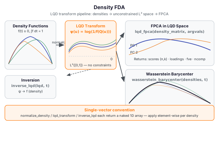
Density FDA treats probability density functions as functional observations and applies functional data analysis techniques to them. The key challenge is that densities live in a constrained Bayes space — they must be non-negative and integrate to one — which rules out standard Euclidean methods. The Log-Quantile-Density (LQD) transform maps each density to an unconstrained \(L^2([0,1])\) function, enabling Euclidean FPCA, regression, and barycenter computation in that transformed space.

Method	`fdars` function	Key output
Normalize to unit integral	`normalize_density`	`(m,)` density
Log-quantile-density transform	`lqd_transform`	`(n_q,)` LQD values on quantile grid
Reconstruct density from LQD	`inverse_lqd`	`(m,)` density on target grid
Geometric mean of densities	`wasserstein_barycenter`	`(m,)` barycenter density
Functional PCA of densities	`lqd_fpca`	scores, loadings, fve (all on quantile grid)

Density FDA — concept diagram

When to use¶

Use density FDA when your data objects are probability distributions rather than ordinary curves. Examples include age-at-death distributions across countries, income distributions across regions, spectral energy distributions of phoneme recordings, or any collection where each observation is a normalized histogram or kernel density estimate.

Why not apply standard FPCA directly to density curves? Raw densities satisfy the non-negativity and unit-integral constraints — pointwise averaging of two valid densities yields a valid density only by chance, and the \(L^2\) metric between densities is not Wasserstein-optimal. The LQD transform sidesteps both issues by mapping each density to an unconstrained \(L^2([0,1])\) function on which ordinary FPCA, regression, and averaging are geometrically correct.

Contrast with Fréchet regression: If your response variable is a density (and your predictors are scalar or Euclidean), use fdars.frechet — see Fréchet Regression. This page covers the case where densities are your primary data objects and you want to summarize, decompose, or compare them via LQD-space FPCA.

Start with normalize_density

Before any LQD operation, run each raw density curve through normalize_density. This converts non-negative values (that need not integrate to 1) to a proper unit density. lqd_transform requires strictly positive input; even a small additive floor (+ 0.01) before normalization avoids division-by-zero at the boundary.

Core Concept¶

Let \(f\) be a probability density on a bounded interval \([a, b]\). Define its quantile function \(Q(u)\) as the inverse of its CDF \(F\). The Log-Quantile-Density (LQD) transform maps \(f\) to:

\[ \psi(u) = \log\!\left(\frac{1}{f(Q(u))}\right), \quad u \in (0, 1) \]

The transformation is invertible via \(f(x) = \exp(-\psi(F(x)))\), and it maps the non-negative constraint of the density space to the unconstrained \(L^2([0,1])\) space. Operations that are not geometrically meaningful in density space — such as pointwise averaging — become correct in LQD space. FPCA in LQD space identifies the principal modes of density shape variation, and the Wasserstein barycenter computes the geometric mean of a collection of densities.

LQD output lives on the quantile grid, not the original argvals grid

lqd_transform(density, argvals) returns an array of length n_q (default max(m, 101)) on the uniform quantile grid \([0, 1]\) — this is not the same length as your input argvals grid of length m. Comparing or combining LQD output with the original grid leads to shape errors.

After calling lqd_transform, construct the quantile grid explicitly before calling inverse_lqd:

psi   = lqd_transform(density, argvals)    # shape (n_q,)
t_q   = np.linspace(0, 1, len(psi))        # the quantile grid
recon = inverse_lqd(psi, t_q, argvals)     # back to shape (m,)

Density Normalization¶

from fdars.density_fda import normalize_density

norm = normalize_density(density, argvals)

Parameter	Type	Description
`density`	`np.ndarray (m,)`	Non-negative density values (need not integrate to 1)
`argvals`	`np.ndarray (m,)`	Evaluation grid

Returns a 1D array (m,) normalized so that \(\int f\,dt \approx 1\). Raises ValueError if any value is negative or if the integral is effectively zero.

LQD Transform and Inverse¶

LQD transform¶

from fdars.density_fda import lqd_transform

psi = lqd_transform(density, argvals, n_quantile_pts=None)

Parameter	Type	Default	Description
`density`	`np.ndarray (m,)`	—	Strictly positive, normalized density
`argvals`	`np.ndarray (m,)`	—	Evaluation grid
`n_quantile_pts`	`int \\| None`	`None`	Quantile grid resolution; `None` uses `max(m, 101)`

Returns a 1D array of shape (n_q,) where n_q = n_quantile_pts or max(m, 101). The output represents \(\psi(u)\) evaluated on the uniform quantile grid np.linspace(0, 1, n_q).

Inverse LQD transform¶

from fdars.density_fda import inverse_lqd

f = inverse_lqd(psi, t_grid, target_argvals)

Parameter	Type	Description
`psi`	`np.ndarray (n_q,)`	LQD values on the quantile grid
`t_grid`	`np.ndarray (n_q,)`	Uniform quantile grid corresponding to `psi`, i.e. `np.linspace(0, 1, len(psi))`
`target_argvals`	`np.ndarray (m,)`	Reconstruction grid — the original argvals

Returns a 1D array (m,) — the reconstructed density on target_argvals.

inverse_lqd requires the explicit quantile grid as second argument

Unlike many inversion routines that take only the transformed values and the target grid, inverse_lqd needs the quantile grid t_grid explicitly — because the quantile grid has length n_q (potentially different from m). Always set t_grid = np.linspace(0, 1, len(psi)) before calling inverse_lqd.

Round-trip fence¶

from fdars.density_fda import normalize_density, lqd_transform, inverse_lqd
import numpy as np

import numpy as np
from fdars.density_fda import normalize_density, lqd_transform, inverse_lqd

rng = np.random.default_rng(42)
m = 50
t = np.linspace(0, 1, m)
raw = np.abs(np.sin(np.pi * t + 0.2)) + 0.01

norm  = normalize_density(raw, t)    # (m,) — valid density
psi   = lqd_transform(norm, t)       # (n_q,) — on the quantile grid, NOT shape (m,)
n_q   = len(psi)
t_q   = np.linspace(0, 1, n_q)      # quantile grid for inverse_lqd
recon = inverse_lqd(psi, t_q, t)    # (m,) — back to original grid

print(f"norm integral:  {np.trapezoid(norm, t):.4f}  (should be ~1.0)")
print(f"psi shape:      {psi.shape}  (quantile grid, n_q={n_q} != m={m})")
print(f"recon integral: {np.trapezoid(recon, t):.4f}  (round-trip, should be ~1.0)")
print("FDARS_FENCE_OK")

norm integral: 1.0000 (should be ~1.0) psi shape: (101,) (quantile grid, n_q=101 != m=50) recon integral: 1.0000 (round-trip, should be ~1.0) FDARS_FENCE_OK

This fence demonstrates the load-bearing correctness proof: psi.shape shows that the LQD output has n_q elements (here 101, since max(50, 101) = 101), confirming it is not the same shape as the m=50 input grid. The round-trip integral close to 1.0 verifies the inversion is accurate.

Wasserstein Barycenter¶

The Wasserstein barycenter computes the geometric mean of a collection of densities in Wasserstein space — the result is the density that minimizes the sum of squared Wasserstein distances to all inputs. Unlike the pointwise average, the Wasserstein barycenter respects the constraint that the result is a valid density, and it interpolates the shape of the input densities rather than their pointwise values.

from fdars.density_fda import wasserstein_barycenter

bary = wasserstein_barycenter(density_matrix, argvals, weights=None)

Parameter	Type	Default	Description
`density_matrix`	`np.ndarray (n, m)`	—	Each row is a normalized density (non-negative, integrating to 1)
`argvals`	`np.ndarray (m,)`	—	Evaluation grid
`weights`	`np.ndarray (n,) \\| None`	`None`	Non-negative weights summing to 1; uniform if `None`

Returns a 1D array (m,) — the Wasserstein barycenter density.

Input rows must be valid unit densities

wasserstein_barycenter requires each row of density_matrix to be non-negative and integrate (approximately) to 1. Always apply normalize_density to each row before stacking them into the matrix. Passing raw, unnormalized density values leads to a barycenter that does not integrate to 1.

LQD-FPCA — Functional PCA of Densities¶

LQD-FPCA applies standard FPCA in the LQD-transformed space, identifying the principal modes of density shape variation. Because the LQD transform is an isometry between the Wasserstein space of densities and \(L^2([0,1])\), the LQD loadings have a direct geometric interpretation: each loading describes a direction of density-shape variation in Wasserstein geometry (e.g. a shift in the mode location, a change in spread).

from fdars.density_fda import lqd_fpca

fp = lqd_fpca(density_matrix, argvals, ncomp=3, n_quantile_pts=None)

Parameter	Type	Default	Description
`density_matrix`	`np.ndarray (n, m)`	—	Each row is a strictly positive, normalized density
`argvals`	`np.ndarray (m,)`	—	Evaluation grid
`ncomp`	`int`	`3`	Number of principal components
`n_quantile_pts`	`int \\| None`	`None`	Quantile grid resolution; `None` uses `max(m, 101)`

Returns — lqd_fpca

Key	Shape	Description
`mean`	`(n_q,)`	Mean LQD function on the quantile grid
`singular_values`	`(ncomp,)`	Singular values
`loadings`	`(n_q, ncomp)`	LQD principal component loadings on the quantile grid
`scores`	`(n, ncomp)`	FPCA scores — use these as features for downstream analysis
`fve`	`(ncomp,)`	Fraction of variance explained (cumulative)
`ncomp`	`int`	Number of retained components

mean and loadings are on the quantile grid (n_q,), not (m,)

The LQD-FPCA results — mean, loadings — are on the quantile grid of length n_q, not the original argvals grid of length m. To visualize a loading against the original domain, use inverse_lqd to map it back. Do not plot fp['loadings'] against the original argvals directly; use np.linspace(0, 1, n_q) as the x-axis or back-transform via inverse_lqd.

Barycenter and LQD-FPCA fence¶

import numpy as np
from fdars.density_fda import normalize_density, lqd_transform, inverse_lqd
from fdars.density_fda import wasserstein_barycenter, lqd_fpca

rng = np.random.default_rng(42)
m, n = 50, 12
t = np.linspace(0.01, 0.99, m)

raw   = np.array([np.abs(np.sin(np.pi * t + rng.uniform(0, 0.5))) + 0.02
                  for _ in range(n)])
norms = np.array([normalize_density(raw[i], t) for i in range(n)])

# Wasserstein barycenter
bary = wasserstein_barycenter(norms, t)

# LQD round-trip on first density
psi_0 = lqd_transform(norms[0], t)          # (n_q,)
n_q   = len(psi_0)
t_q   = np.linspace(0, 1, n_q)
recon = inverse_lqd(psi_0, t_q, t)          # (m,) round-trip

# LQD-FPCA over all densities
fp = lqd_fpca(norms, t, ncomp=2)

print(f"norm integral (density 0): {np.trapezoid(norms[0], t):.4f}")
print(f"recon integral (round-trip): {np.trapezoid(recon, t):.4f}")
print(f"barycenter integral: {np.trapezoid(bary, t):.4f}")
print(f"lqd_fpca scores shape: {np.asarray(fp['scores']).shape}  (n, ncomp)")
print(f"fve (cumulative): {np.asarray(fp['fve']).round(3).tolist()}")
print("FDARS_FENCE_OK")

norm integral (density 0): 1.0000 recon integral (round-trip): 1.0000 barycenter integral: 1.0000 lqd_fpca scores shape: (12, 2) (n, ncomp) fve (cumulative): [0.798, 1.0] FDARS_FENCE_OK

Parameter Selection and Result Interpretation¶

Choosing `ncomp` via `fve`¶

The fve key in lqd_fpca gives the cumulative fraction of variance explained. Use it to select ncomp:

fp  = lqd_fpca(density_matrix, argvals, ncomp=10)
fve = np.asarray(fp["fve"])                  # cumulative FVE per component
ncomp_choice = int(np.argmax(fve >= 0.90)) + 1
print(f"Components for 90% FVE: {ncomp_choice}")

A typical density population is well-explained by 2–4 components (the dominant modes are location, scale, and skewness shifts). If the first component explains > 80% of variance, the collection has little density-shape variation and a single component suffices.

Reading LQD loadings¶

Each column of fp['loadings'] (shape (n_q, ncomp)) is a function on the uniform quantile grid \([0, 1]\). Positive values of a loading at quantile \(u\) mean that densities with high scores on that component have more probability mass in the region around quantile \(u\). A loading that shifts from negative to positive across the quantile range corresponds to a location (mode) shift in the original density space.

Using scores downstream¶

The scores matrix (n, ncomp) is the natural feature representation for downstream tasks — clustering, classification, regression with scalar predictors. Because the LQD transform is an isometry, distances in score space approximate Wasserstein distances between the original densities.

Density visualization fence¶

import numpy as np
from docs_fig import fig, render
from fdars.density_fda import normalize_density, wasserstein_barycenter, lqd_fpca

rng = np.random.default_rng(42)
m, n = 60, 10
t = np.linspace(0.01, 0.99, m)

# Simulate densities with varying mode locations
raw   = np.array([
    np.abs(np.sin(np.pi * t + rng.uniform(0.1, 1.0))) + 0.02
    for _ in range(n)
])
norms = np.array([normalize_density(raw[i], t) for i in range(n)])
bary  = wasserstein_barycenter(norms, t)
fp    = lqd_fpca(norms, t, ncomp=2)

f, axes = fig(1, 2, figsize=(11.0, 4.0))

# Left: individual densities + barycenter
ax = axes[0]
for i, d in enumerate(norms):
    ax.plot(t, d, color="#6c757d", lw=0.9, alpha=0.4, label="_")
ax.plot(t, bary, color="#e8710a", lw=2.4, label="Wasserstein barycenter")
ax.set(title="Density sample + Wasserstein barycenter",
       xlabel="t", ylabel="density")
ax.legend()

# Right: LQD-FPCA score scatter (2 components)
scores = np.asarray(fp["scores"])
fve    = np.asarray(fp["fve"])
ax2 = axes[1]
ax2.scatter(scores[:, 0], scores[:, 1], color="#3f51b5", s=60, edgecolors="white", lw=0.6)
ax2.set(title=f"LQD-FPCA score scatter\nFVE: {fve[0]:.0%} + {fve[1]-fve[0]:.0%}",
        xlabel="PC1 score", ylabel="PC2 score")
ax2.axhline(0, color="#6c757d", lw=0.7, ls="--")
ax2.axvline(0, color="#6c757d", lw=0.7, ls="--")

print(render(f))
print("FDARS_FENCE_OK")

FDARS_FENCE_OK

Methods available in R but not yet in Python¶

Fréchet regression on density responses — if the response variable is a density, use fdars.frechet which provides frechet_global_reg for Wasserstein regression. See Fréchet Regression for the full API.
Density-on-scalar regression beyond Fréchet global — fitting a flexible nonlinear regression of density responses on scalar predictors is not directly exposed in fdars beyond frechet_global_reg.

References¶

Petersen, A. and Müller, H.-G. (2016). Functional data analysis for density functions by transformation to a Hilbert space. Annals of Statistics 44(1), 183–218.
van den Boogaart, K. G., Egozcue, J. J. and Pawlowsky-Glahn, V. (2014). Bayes Hilbert spaces. Australian & New Zealand Journal of Statistics 56(2), 171–194.