Additive Scalar-on-Function Regression¶

Additive Scalar-on-Function (SoF) regression predicts a scalar response from one or more functional predictors by decomposing the functional effect into a sum of smooth component functions. This is a nonparametric generalization of the classical linear SoF model that allows each predictor to contribute a non-linear partial effect while keeping the model interpretable.

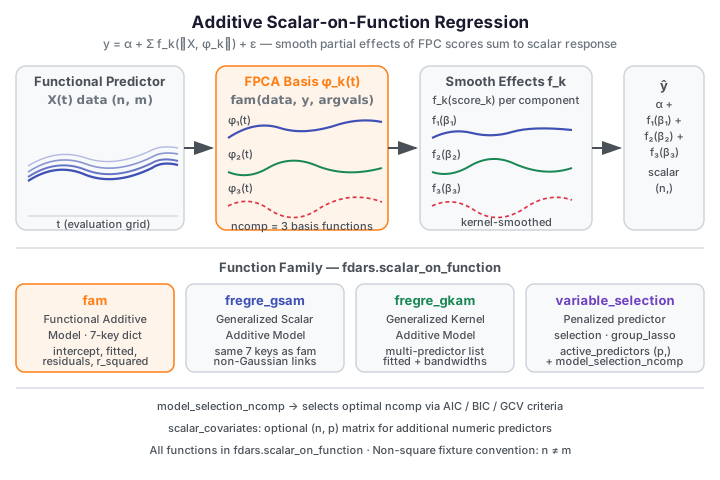
Additive Scalar-on-Function Regression — concept diagram

Let \(y_i\) be a scalar response and \(X_{ij}(t)\) be the \(j\)-th functional predictor for observation \(i\). The additive SoF model takes the form:

\[ y_i = \alpha + \sum_{j=1}^{p} f_j\!\left(\langle X_{ij}, \phi_j \rangle\right) + \varepsilon_i \]

where \(\phi_j\) are the leading FPCA basis functions for predictor \(j\) and each \(f_j\) is a smooth function of the corresponding FPC scores. The Functional Additive Model (FAM) estimates these smooth components jointly, providing a flexible alternative to simple linear projection while remaining far more parsimonious than a fully nonparametric approach.

Module path

All functions on this page are in the fdars.scalar_on_function submodule, not fdars.regression. Use from fdars.scalar_on_function import fam, fregre_gsam, fregre_gkam, variable_selection, model_selection_ncomp.

When to use¶

Method	`fdars` function	Key idea	Best when
Functional Additive Model	`fam`	FPCA + smooth additive effects per component	Single functional predictor; non-linear but smooth relationship
Generalized Structured Additive	`fregre_gsam`	Same as FAM; identical interface	Non-Gaussian responses or alternative link; same single-predictor case
Generalized Kernel Additive	`fregre_gkam`	Kernel regression directly on curves, no FPCA	Multiple functional predictors; backfitting over kernels
Variable selection	`variable_selection`	Group-LASSO over FPC projections	Many predictors; want to identify the active subset
Component count selection	`model_selection_ncomp`	AIC/BIC/GCV over candidate component counts	Tuning `ncomp` before fitting `fam` or `fregre_gsam`

Start with fam or fregre_gsam for a single functional predictor. They share the same 7-key interface and both auto-select ncomp and bandwidth via GCV when the defaults ncomp=0, bandwidth=0.0 are left in place.

Switch to fregre_gkam when you have multiple functional predictors — its backfitting algorithm fits each predictor's additive effect in turn.

Use variable_selection when predictors are many and sparsity is expected; the group-LASSO penalty zeros out uninformative predictor blocks entirely.

Link to the linear baseline: Scalar-on-Function Regression.

1. FAM — Functional Additive Model¶

fam fits a functional additive model with a single functional predictor. It projects the predictor onto its leading FPCA components and estimates a smooth additive effect for each component score.

from fdars.scalar_on_function import fam

result = fam(data, y, argvals,
             scalar_covariates=None,
             ncomp=0,            # 0 = auto via GCV
             bandwidth=0.0,      # 0.0 = auto per component via GCV
             kernel="gaussian",
             n_grid_bandwidth=20)

Auto-selection defaults: ncomp=0 and bandwidth=0.0

The default values are ncomp=0 (auto via GCV) and bandwidth=0.0 (auto per component via GCV). Older documentation incorrectly listed defaults of ncomp=3 and bandwidth=0.5 — these are wrong. Pass explicit values only when you want to fix the tuning rather than letting GCV select it.

Parameter	Type	Default	Description
`data`	`np.ndarray (n, m)`	—	Functional predictor observations
`y`	`np.ndarray (n,)`	—	Scalar response vector
`argvals`	`np.ndarray (m,)`	—	Evaluation grid
`scalar_covariates`	`np.ndarray (n, q)` or `None`	`None`	Optional additional scalar predictors
`ncomp`	`int`	`0`	Number of FPCA components (0 = auto via GCV)
`bandwidth`	`float`	`0.0`	Bandwidth for smooth component estimator (0.0 = auto via GCV)
`kernel`	`str`	`"gaussian"`	Kernel type: `"gaussian"`, `"epanechnikov"`, `"tricube"`
`n_grid_bandwidth`	`int`	`20`	Bandwidth grid size for GCV selection

Return dict (7 keys):

Key	Type	Description
`fitted_values`	`np.ndarray (n,)`	Fitted scalar responses, one per observation
`residuals`	`np.ndarray (n,)`	Raw residuals
`component_fits`	`list` of `np.ndarray (n,)`	Per-FPC smooth partial effects, one array per component
`intercept`	`float`	Model intercept
`bandwidths`	`np.ndarray (ncomp,)`	Selected bandwidth per FPCA component
`ncomp`	`int`	Number of FPCA components actually used (after GCV if `ncomp=0`)
`r_squared`	`float`	Global R²

import numpy as np
from fdars.scalar_on_function import fam

rng = np.random.default_rng(42)
n, m = 25, 30
t = np.linspace(0, 1, m)
data = np.array([np.sin(2 * np.pi * t + rng.uniform(0, 0.5)) for _ in range(n)])
y = np.array([np.trapezoid(data[i] ** 2, t) + 0.1 * rng.standard_normal() for i in range(n)])

result = fam(data, y, t, ncomp=3, bandwidth=0.5)
print(f"ncomp used:      {result['ncomp']}")
print(f"r_squared:       {result['r_squared']:.4f}")
print(f"fitted shape:    {np.asarray(result['fitted_values']).shape}")
print(f"bandwidths:      {np.round(np.asarray(result['bandwidths']), 3)}")
print("FDARS_FENCE_OK")

ncomp used: 3 r_squared: 0.0002 fitted shape: (25,) bandwidths: [0.5 0.5 0.5] FDARS_FENCE_OK

2. `fregre_gsam` — Generalized Structured Additive Model¶

fregre_gsam shares the exact same signature and return structure as fam — 7 identical keys. It uses a generalized additive framework that can accommodate non-Gaussian responses through a link function.

from fdars.scalar_on_function import fregre_gsam

result = fregre_gsam(data, y, argvals,
                     scalar_covariates=None,
                     ncomp=0,            # 0 = auto via GCV
                     bandwidth=0.0,      # 0.0 = auto per component via GCV
                     kernel="gaussian",
                     n_grid_bandwidth=20)

The returned dict has the same 7 keys as fam: fitted_values, residuals, component_fits, intercept, bandwidths, ncomp, r_squared.

FAM vs GSAM

For Gaussian responses, fam and fregre_gsam produce similar fits. Prefer fregre_gsam when a non-identity link function is appropriate for your response distribution.

3. `fregre_gkam` — Generalized Kernel Additive Model¶

fregre_gkam fits additive effects using kernel regression directly on the raw functional curves, without an intermediate FPCA step. It handles multiple functional predictors simultaneously via a backfitting algorithm.

from fdars.scalar_on_function import fregre_gkam

result = fregre_gkam(predictors, y, argvals_list,
                     scalar_covariates=None,
                     bandwidth=0.0,      # 0.0 = auto per predictor via GCV
                     kernel="gaussian",
                     max_iter=50,
                     epsilon=1e-6)

Parameter	Type	Default	Description
`predictors`	`list` of `np.ndarray (n, m_p)`	—	One array per functional predictor
`y`	`np.ndarray (n,)`	—	Scalar response
`argvals_list`	`list` of `np.ndarray (m_p,)`	—	Evaluation grid per predictor
`scalar_covariates`	`np.ndarray (n, q)` or `None`	`None`	Optional scalar predictors
`bandwidth`	`float`	`0.0`	Kernel bandwidth (0.0 = auto per predictor via GCV)
`kernel`	`str`	`"gaussian"`	Kernel type
`max_iter`	`int`	`50`	Maximum backfitting iterations
`epsilon`	`float`	`1e-6`	Convergence tolerance

Return dict (8 keys):

Key	Type	Description
`fitted_values`	`np.ndarray (n,)`	Fitted scalar responses
`residuals`	`np.ndarray (n,)`	Raw residuals
`component_fits`	`list` of `np.ndarray (n,)`	Per-predictor partial effects
`intercept`	`float`	Model intercept
`bandwidths`	`np.ndarray (P,)`	Selected bandwidth per predictor
`iterations`	`int`	Number of backfitting iterations performed
`converged`	`bool`	Whether backfitting reached the convergence tolerance
`r_squared`	`float`	Global R²

GKAM backfitting convergence

Always check result['converged'] after calling fregre_gkam. If converged is False, try increasing max_iter (default 50) or loosening epsilon (default 1e-6). The number of iterations performed is in result['iterations']. With many predictors, backfitting may be slow — reduce max_iter during exploration and then confirm convergence with the full budget.

import numpy as np
from fdars.scalar_on_function import fregre_gkam

rng = np.random.default_rng(7)
n, m = 25, 20
t = np.linspace(0, 1, m)

# Two functional predictors
x1 = np.array([np.sin(2 * np.pi * t + rng.uniform(0, 0.3)) for _ in range(n)])
x2 = np.array([np.cos(np.pi * t + rng.uniform(0, 0.5)) for _ in range(n)])
y = (np.array([np.trapezoid(x1[i], t) for i in range(n)])
     + 0.5 * np.array([np.trapezoid(x2[i] ** 2, t) for i in range(n)])
     + 0.1 * rng.standard_normal(n))

result = fregre_gkam([x1, x2], y, [t, t], bandwidth=0.3, max_iter=50)

print(f"converged:    {result['converged']}")
print(f"iterations:   {result['iterations']}")
print(f"r_squared:    {result['r_squared']:.4f}")
print(f"bandwidths:   {np.round(np.asarray(result['bandwidths']), 3)}")
print(f"n_components: {len(result['component_fits'])}")
print("FDARS_FENCE_OK")

converged: False iterations: 50 r_squared: 0.0004 bandwidths: [0.3 0.3] n_components: 2 FDARS_FENCE_OK

4. `variable_selection` — Predictor Selection¶

For multi-predictor settings, variable_selection identifies which functional predictors are relevant using a penalized FPCA projection regression.

from fdars.scalar_on_function import variable_selection

sel = variable_selection(predictors, y, argvals_list,
                         scalar_covariates=None,
                         ncomp=3,
                         penalty="group_lasso",
                         lambda_=0.0,         # 0.0 = auto via lambda grid
                         max_iter=100,
                         epsilon=1e-5,
                         lambda_n_grid=20)

Parameter	Type	Default	Description
`predictors`	`list` of `np.ndarray (n, m_p)`	—	One array per functional predictor
`y`	`np.ndarray (n,)`	—	Scalar response
`argvals_list`	`list` of `np.ndarray (m_p,)`	—	Evaluation grid per predictor
`ncomp`	`int`	`3`	Number of FPCA components per predictor
`penalty`	`str`	`"group_lasso"`	Penalty type: `"group_lasso"` or `"ls"`
`lambda_`	`float`	`0.0`	Regularization strength (0.0 = auto via grid)
`max_iter`	`int`	`100`	Maximum iterations
`epsilon`	`float`	`1e-5`	Convergence tolerance
`lambda_n_grid`	`int`	`20`	Lambda grid points for auto selection

Return dict (9 keys):

Key	Type	Description
`active_predictors`	`np.ndarray (P,)` bool	`True` for each predictor selected by the penalty
`coefficients`	`list` of `np.ndarray`	Estimated FPCA coefficient vectors, one per predictor
`fitted_values`	`np.ndarray (n,)`	Fitted scalar responses
`residuals`	`np.ndarray (n,)`	Raw residuals
`intercept`	`float`	Model intercept
`lambda`	`float`	Regularization strength used (auto-selected if `lambda_=0.0`)
`r_squared`	`float`	Global R²
`iterations`	`int`	Iterations performed by the optimization
`converged`	`bool`	Whether the optimization converged

Supported penalties: "group_lasso" and "ls" only. Penalties "group_mcp" and "group_scad" raise ValueError (not yet implemented in fdars-core 0.33).

5. `model_selection_ncomp` — Component Count Selection¶

Selects the optimal number of FPCA components using information criteria, useful for tuning ncomp before a FAM or GSAM fit.

from fdars.scalar_on_function import model_selection_ncomp

ms = model_selection_ncomp(data, response, max_comp=10, criterion="gcv")

Use max_comp — not the old name

The parameter controlling the maximum component count is named max_comp. Older documentation used a different name; using the old spelling as a keyword argument raises TypeError. Pass the value as max_comp=10.

Parameter	Type	Default	Description
`data`	`np.ndarray (n, m)`	—	Functional predictor
`response`	`np.ndarray (n,)`	—	Scalar response
`max_comp`	`int`	`10`	Maximum number of components to evaluate
`criterion`	`str`	`"gcv"`	Selection criterion: `"aic"`, `"bic"`, or `"gcv"`

Return dict (2 keys):

Key	Type	Description
`best_ncomp`	`int`	Optimal component count per the chosen criterion
`criteria`	`list` of `(ncomp, aic, bic, gcv)` tuples	Criterion values for each candidate count

6. Parameter Selection¶

Choosing `ncomp` and `bandwidth` for `fam` / `fregre_gsam`¶

Leave both at their defaults (ncomp=0, bandwidth=0.0) to let GCV choose automatically. Use model_selection_ncomp beforehand if you want an explicit criterion-comparison table:

import numpy as np
from fdars.scalar_on_function import model_selection_ncomp

rng = np.random.default_rng(42)
n, m = 30, 30
t = np.linspace(0, 1, m)
data = np.array([np.sin(2 * np.pi * t + rng.uniform(0, 0.5)) for _ in range(n)])
y = np.array([np.trapezoid(data[i] ** 2, t) + 0.1 * rng.standard_normal() for i in range(n)])

ms = model_selection_ncomp(data, y, max_comp=8, criterion="gcv")
print(f"best_ncomp (GCV): {ms['best_ncomp']}")
print("ncomp | AIC    | BIC    | GCV")
for row in ms["criteria"]:
    print(f"  {row[0]:2d}  | {row[1]:.4f} | {row[2]:.4f} | {row[3]:.4f}")
print("FDARS_FENCE_OK")

best_ncomp (GCV): 1 ncomp | AIC | BIC | GCV 1 | -148.2950 | -145.4926 | 0.0073 2 | -146.2952 | -142.0916 | 0.0082 FDARS_FENCE_OK

Backfitting convergence for `fregre_gkam`¶

The GKAM backfitting algorithm cycles through predictors, updating each partial effect while holding the others fixed. Check result['converged'] and result['iterations'] after every fit. Typical convergence requires 10–30 iterations for 2–5 predictors. Increase max_iter if convergence is slow; widen epsilon slightly if the algorithm cycles without converging.

7. Result Interpretation¶

Component fits — partial effects per predictor¶

component_fits in all three models (fam, fregre_gsam, fregre_gkam) is a Python list of 1-D arrays, one per FPCA component (FAM/GSAM) or per predictor (GKAM). Each array has length n and contains the fitted partial effect for that component across all observations.

For fam and fregre_gsam: component_fits[k] is the contribution of the k-th FPCA score to the fitted value. Plot them against the corresponding FPCA score to see the shape of the smooth function \(f_k\).

For fregre_gkam: component_fits[k] is the fitted partial effect of the k-th functional predictor. Plotting each array shows how much each predictor contributes to the fit.

Interpreting `active_predictors` from `variable_selection`¶

active_predictors is a boolean array of length P (number of predictors). A True entry means the group-LASSO penalty kept that predictor's coefficient block non-zero — it is considered informative. False means the penalty drove that block to zero.

Choosing lambda_: smaller values retain more predictors; larger values remove more. With lambda_=0.0 (default), the function searches a grid of 20 lambda values (lambda_n_grid=20) and picks the one that minimizes the penalized criterion. Inspect result['lambda'] to see the chosen value.

8. Figure: Partial-Effect Curves from FAM¶

import numpy as np
from docs_fig import fig, render
from fdars.scalar_on_function import fam

rng = np.random.default_rng(42)
n, m = 30, 40
t = np.linspace(0, 1, m)

# Functional predictor: sine waves with random phase
data = np.array([np.sin(2 * np.pi * t + rng.uniform(0, 0.8)) for _ in range(n)])
# Response: nonlinear in the L2 norm of the curve
y = np.array([np.trapezoid(data[i] ** 2, t) + 0.05 * rng.standard_normal() for i in range(n)])

result = fam(data, y, t, ncomp=3, bandwidth=0.5)

# Plot partial-effect contributions (component_fits) for the first 3 FPCs
# sorted by the FPC scores to reveal the smooth function shape

# Compute FPC scores to sort along x-axis
cfs = result["component_fits"]
ncomp_used = result["ncomp"]

f, ax = fig()
colors = ["#3f51b5", "#e8710a", "#198754"]
for k in range(min(ncomp_used, 3)):
    cf = np.asarray(cfs[k])
    # Sort by component_fit value to plot the smooth curve cleanly
    order = np.argsort(cf)
    label = f"Component {k+1}"
    ax.plot(np.arange(n)[order] / n, cf[order], color=colors[k], lw=2, label=label)
ax.set(
    title="FAM partial-effect curves per FPCA component",
    xlabel="Observation rank (sorted by component fit)",
    ylabel="Partial effect contribution",
)
ax.legend()
print(render(f))
print("FDARS_FENCE_OK")

FDARS_FENCE_OK

Methods available in the R package but not (yet) in Python¶

Methods available in the R package but not (yet) in Python

The "group_mcp" and "group_scad" penalty options for variable_selection are not yet implemented in fdars-core 0.33 — passing them raises ValueError. Only "group_lasso" and "ls" are supported.

References¶

Müller, H.-G. and Yao, F. (2008). Functional additive models. Journal of the American Statistical Association 103(484), 1534–1544.
Fan, J. and Zhang, J.-T. (2000). Two-step estimation of functional linear models with applications to longitudinal data. Journal of the Royal Statistical Society B 62(2), 303–322.
Marx, B. D. and Eilers, P. H. C. (1999). Generalized linear regression on sampled signals and curves: A P-spline approach. Technometrics 41(1), 1–13.

Additive Scalar-on-Function Regression¶

When to use¶

1. FAM — Functional Additive Model¶

2. fregre_gsam — Generalized Structured Additive Model¶

3. fregre_gkam — Generalized Kernel Additive Model¶

4. variable_selection — Predictor Selection¶

5. model_selection_ncomp — Component Count Selection¶